5步掌握贝叶斯优化：高效调优你的XGBoost模型（附源码）

XGBoost作为一种典型的机器学习数学模型（eXtreme Gradient Boosting）是一个高效、可扩展的机器学习库，基于梯度提升树（Gradient Boosted Trees）算法，通过迭代构建树模型并对误差进行拟合来提升预测精度。它通过引入正则化、列抽样、近似分裂点、多线程并行和分布式计算等优化，显著提高了模型性能和计算效率，广泛应用于分类、回归和排序等任务。XGBoost 尤其在处理大规模表格数据中表现突出。在kaggle竞赛中有着补课或缺的重要性，也因此获得了广泛的关注。

数学原理

假设我们训练了K棵树，那么对于第i个样本的最终预测值应当为:

已知训练数据集为T={{(x_1,y_1),(x_2,y_2),(x_3,y_3)...}}，损失函数为l(y_i, \hat{y}_i),正则化项是\Omega(f_k)。那么整体目标函数可以表示成如下的形式:

其中，

1. 我们记\sum_k \Omega(f_k) 表示k棵树的复杂程度。

2. L（emptyset）是线性空间上的表达

3. \hat{y}_i是第i个样本中的x_i预测值

下面用GBDT提升树表达XGboost，由于\hat{y}_i 可以用GBDT梯度提升树方式进行表达:\hat{y}_i = \sum_{k=1}^{K} f_k(x_i) = \hat{y}_i^{(t-1)} + f_t(x_i)

于是将\mathcal{L}(\emptyset)转化为如下形式:

这便是XGboost最优化函数的表达形式，接下来分三个步骤优化此函数。

STEP 1：二阶泰勒展开，去除常数项，优化损失函数项

假设l(x)=l(y_1,x)，则对l(y_1,x)在x_0处进行二阶泰勒展开得到:

同理，将l(y_1,x) 在\hat{y}_i^{(t-1)}处泰勒展开，

其中\hat{y}_i^{(t-1)} 是一个已知的量，不妨令x = \hat{y}_i^{(t-1)} + f_t(x_i)，且记一阶导为g_i = l'(y_i, \hat{y}_i^{(t-1)})，二阶导为h_i = l''(y_i, \hat{y}_i^{(t-1)})

得到的l(y_i, \hat{y}_i^{(t-1)} + f_t(x_i))二阶泰勒展开，得到:

带入原来的目标函数，我们可以等得到其表达式可以简化为:

至此我们便将其中的常数项干扰项全部消去了，达到了简化的目标。

STEP 2:正则化展开，去除常数项

由于l(y_i, \hat{y}_i^{(t-1)} + f_t(x_i)) 是一个常数项，对最优化是不起到任何影响的，所以考虑移除之，化简得到:

将其正则化拆分得到:

其中，\sum_{k=1}^{t-1} \Omega(f_k)是一个常数，又由于在计算第t棵树的时候，前t-1棵树的结构式已经确定的，因此也是可以记作成一个常数的，其具体表达式如下;

将上式最右端的常数去掉，便可得到下面的表达式:

STEP 3:合并一次项、二次项系数

新定义一个树，将属于第j个叶子结点的所有样本x_j,划入到一个叶子结点中，数学描述如下:

对于STEP2中化简得到的\mathcal{L}^{(t)} = \sum_{i=1}^{n} \left[ g_i f_t(x_i) + \frac{1}{2} h_i f_t^2(x_i) \right] + \Omega(f_t)，将f_t(x_i) = w_{q(x_i)}代入原目标函数，有:

将所有的训练样本，按叶子结点进行分组得到:

最后合并一次项和二次项系数"

定义G_j = \sum_{i \in I_j} g_i \qquad H_j = \sum_{i \in I_j} h_i

其中，Gj指的是叶子结点j所包含样本的一节偏导数之和，因此是一个常数，而Hj表示的是叶子结点j所包含样本的一节偏导数之和，因此也是一个常数，将Gj与Hj代入原来的目标函数表达式，得到XGboost最终的目标优化函数:

最优解的求解

XGBoost目标函数的各个叶子结点的目标式子是相互独立的。即每个叶子结点的式子都达到最值点，整个目标函数也达到最值点。则每个叶子的权重节点以及此时最优的OBJ函数值为:

在实际训练xgboost时，最佳分裂点是一个关键问题，常用的方法如下:贪心算法与近似算法。

代码实现

XGboost最常出现用于数据特征挖掘分析，例如下面的例子，以探究糖尿病的影响因素，以'diabetes.csv’数据库为例，以其编写的xgboost代码如下:

数据库的下载如下:Machine-Learning-with-Python/diabetes.csv at master · susanli2016/Machine-Learning-with-Python

需要注意的是XGboost需要不断地调整参数，先大范围的进行调整，随后再粗略范围内进行微小波动调整。

import pandas as pd
from sklearn import metrics
from sklearn.model_selection import train_test_split
import xgboost as xgb
import matplotlib.pyplot as plt

plt.rcParams['font.sans-serif'] = ['SimHei']  # 设置中文黑体
plt.rcParams['axes.unicode_minus'] = False    # 正常显示负号

# 导入数据集
df = pd.read_csv(r"C:\Users\asus\Downloads\diabetes.csv")
data=df.iloc[:,:8]
target=df.iloc[:,-1]
 
# 切分训练集和测试集
train_x, test_x, train_y, test_y = train_test_split(data,target,test_size=0.2,random_state=7)

# xgboost模型初始化设置
dtrain=xgb.DMatrix(train_x,label=train_y)
dtest=xgb.DMatrix(test_x)
watchlist = [(dtrain,'train')]

# booster:
params={'booster':'gbtree',
        'objective': 'binary:logistic',
        'eval_metric': 'auc',
        'max_depth':5,
        'lambda':10,
        'subsample':0.75,
        'colsample_bytree':0.75,
        'min_child_weight':2,
        'eta': 0.025,
        'seed':0,
        'nthread':8,
        'gamma':0.15,
        'learning_rate' : 0.01}

# 建模与预测：50棵树
bst=xgb.train(params,dtrain,num_boost_round=50,evals=watchlist)
ypred=bst.predict(dtest)
 
# 设置阈值、评价指标
y_pred = (ypred >= 0.5)*1
print ('Precesion: %.4f' %metrics.precision_score(test_y,y_pred))
print ('Recall: %.4f' % metrics.recall_score(test_y,y_pred))
print ('F1-score: %.4f' %metrics.f1_score(test_y,y_pred))
print ('Accuracy: %.4f' % metrics.accuracy_score(test_y,y_pred))
print ('AUC: %.4f' % metrics.roc_auc_score(test_y,ypred))

ypred = bst.predict(dtest)
print("测试集每个样本的得分\n",ypred)
ypred_leaf = bst.predict(dtest, pred_leaf=True)
print("测试集每棵树所属的节点数\n",ypred_leaf)
ypred_contribs = bst.predict(dtest, pred_contribs=True)
print("特征的重要性\n",ypred_contribs )

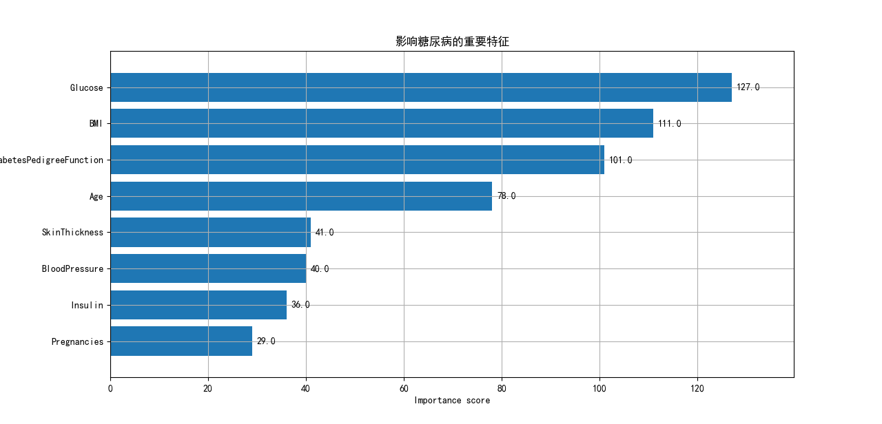
xgb.plot_importance(bst,height=0.8,title='影响糖尿病的重要特征', ylabel='特征')
plt.rc('font', family='Arial Unicode MS', size=14)
plt.show()

在运行完python代码后，便可得到如下的结果，容易知道，血液中葡萄糖含量是其重要的影响因素。

基于贝叶斯优化对XGboost参数的调整

将贝叶斯优化应用于 XGBoost 参数调优的具体流程如下：

1.定义参数空间：确定需要优化的 XGBoost 参数及其取值范围，例如：

• learning_rate：学习率，通常在 [0.01, 0.3] 范围内

• max_depth：树的最大深度，通常在 [3, 10] 范围内

• min_child_weight：叶子节点所需的最小样本权重和，通常在 [1, 10] 范围内

• gamma：在节点分裂时所需的最小损失函数减少量，通常在 [0, 1] 范围内

• subsample：训练每棵树时使用的样本比例，通常在 [0.5, 1] 范围内

• colsample_bytree：构建每棵树时使用的特征比例，通常在 [0.5, 1] 范围内

• lambda：L2 正则化项，通常在 [0.1, 10] 范围内

• alpha：L1 正则化项，通常在 [0, 10] 范围内

2.定义目标函数：通常是交叉验证的性能指标（如准确率、AUC、RMSE 等）的负值（因为贝叶斯优化默认是最小化问题）。

3. 初始化：随机选择几个初始点，评估其性能，并用这些点初始化高斯过程模型。

4. 迭代优化：

• 使用当前的观测数据更新高斯过程模型

• 使用采集函数确定下一个最有希望的参数组合

• 使用新的参数组合训练 XGBoost 模型并评估性能

• 将新的观测结果添加到数据集中

• 重复上述步骤，直到达到预定的迭代次数或满足停止条件

5. 选择最优参数：从所有评估过的参数组合中选择性能最好的一组作为最终结果。

高斯过程是贝叶斯优化的一种常用的概率模型，可以看作是定义在函数空间上的多元高斯分布的扩展。对于任意有限的输入点集合，函数值的联合分布是多元高斯分布。

高斯过程由均值函数m(x) 和协方差函数（核函数）k(x, x')完全确定：

通常，均值函数被设为零，而核函数则描述了不同输入点之间函数值的相关性。常用的核函数包括径向基函数（RBF）核、Matérn核等。

给定观测数据D = \{(x_i, y_i)\}_{i=1}^n，高斯过程可以用于预测新输入点x_* 的函数值分布：

其中，预测均值和方差分别为：

这里，X是观测输入点的集合，Y是对应的观测值，K(X,X)是观测点之间的核矩阵，\sigma_n^2是观测噪声方差。

采集函数用于在贝叶斯优化过程中选择下一个评估点。以期望改进（EI）为例，其定义为：

其中f(x^+) 是当前观测到的最优函数值。EI可以解析计算为：

其中，Z = \frac{\mu(x) - f(x^+)}{\sigma(x)}，\Phi 和\phi 分别是标准正态分布的累积分布函数和概率密度函数。

相比网格搜索和随机搜索，贝叶斯优化通常需要更少的迭代次数就能找到较好的参数组合，大大节省计算资源。

基于贝叶斯参数优化之后的python代码如下:

import numpy as np
import pandas as pd
import matplotlib.pyplot as plt
from sklearn.datasets import fetch_california_housing
from sklearn.model_selection import train_test_split, cross_val_score
from sklearn.metrics import mean_squared_error, r2_score
import xgboost as xgb
from skopt import BayesSearchCV
from skopt.space import Real, Integer
import warnings
import time
warnings.filterwarnings('ignore')

plt.rcParams['font.sans-serif'] = ['SimHei']  # 设置中文黑体
plt.rcParams['axes.unicode_minus'] = False    # 正常显示负号

# 加载加利福尼亚房价数据集（回归问题）
print("加载数据集...")
data = fetch_california_housing()
X = pd.DataFrame(data.data, columns=data.feature_names)
y = data.target

# 为了加速演示，使用部分数据
print("准备数据集（使用部分数据以加速演示）...")
X_sample = X.sample(n=5000, random_state=42)
y_sample = y[X_sample.index]

# 划分训练集和测试集
X_train, X_test, y_train, y_test = train_test_split(X_sample, y_sample, test_size=0.2, random_state=42)

print(f"训练集大小: {X_train.shape}")
print(f"测试集大小: {X_test.shape}")

print("\n开始贝叶斯优化参数调整...")
print("=" * 50)

# 定义参数搜索空间（减少搜索范围以加速）
param_space = {
    'n_estimators': Integer(50, 200),  # 减少上限
    'learning_rate': Real(0.05, 0.3, prior='log-uniform'),
    'max_depth': Integer(3, 8),  # 减少上限
    'subsample': Real(0.7, 1.0),
    'colsample_bytree': Real(0.7, 1.0),
    'reg_alpha': Real(0, 5),  # 减少上限
    'reg_lambda': Real(1, 5)  # 减少上限
}

# 创建XGBoost模型（移除early_stopping以避免错误）
xgb_model = xgb.XGBRegressor(
    random_state=42, 
    n_jobs=-1,
    eval_metric='rmse'
)

print("配置贝叶斯搜索...")
# 贝叶斯优化（减少迭代次数）
bayes_search = BayesSearchCV(
    estimator=xgb_model,
    search_spaces=param_space,
    n_iter=15,  # 进一步减少迭代次数
    cv=3,       # 减少交叉验证折数
    scoring='neg_root_mean_squared_error',
    n_jobs=1,   # 改为单进程避免冲突
    random_state=42,
    verbose=1   # 减少输出详细程度
)

# 执行优化
print("开始优化过程...")
start_time = time.time()

try:
    bayes_search.fit(X_train, y_train)
    
    optimization_time = time.time() - start_time
    print(f"\n优化完成！耗时: {optimization_time:.2f} 秒")
    print("=" * 50)
    print(f"最佳参数: {bayes_search.best_params_}")
    print(f"最佳CV分数: {-bayes_search.best_score_:.4f}")

    # 使用最优参数训练最终模型
    best_model = bayes_search.best_estimator_

    # 在测试集上进行预测
    y_pred = best_model.predict(X_test)

    # 评估模型性能
    mse = mean_squared_error(y_test, y_pred)
    rmse = np.sqrt(mse)
    r2 = r2_score(y_test, y_pred)

    print("\n优化后模型性能:")
    print("=" * 30)
    print(f"均方误差 (MSE): {mse:.4f}")
    print(f"均方根误差 (RMSE): {rmse:.4f}")
    print(f"决定系数 (R²): {r2:.4f}")

    # 对比默认参数模型
    print("\n训练默认参数模型进行对比...")
    default_model = xgb.XGBRegressor(
        n_estimators=100,
        learning_rate=0.1,
        max_depth=3,
        random_state=42
    )
    default_model.fit(X_train, y_train)
    y_pred_default = default_model.predict(X_test)
    rmse_default = np.sqrt(mean_squared_error(y_test, y_pred_default))
    r2_default = r2_score(y_test, y_pred_default)

    print("\n默认参数模型性能:")
    print("=" * 30)
    print(f"均方根误差 (RMSE): {rmse_default:.4f}")
    print(f"决定系数 (R²): {r2_default:.4f}")

    print(f"\n性能提升:")
    print("=" * 20)
    print(f"RMSE 改善: {((rmse_default - rmse) / rmse_default * 100):.2f}%")
    print(f"R² 改善: {((r2 - r2_default) / r2_default * 100):.2f}%")

    # 查看特征重要性
    importance = best_model.feature_importances_
    feature_names = X.columns

    # 可视化特征重要性
    indices = np.argsort(importance)[::-1]

    print("\n生成可视化图表...")
    plt.figure(figsize=(12, 8))

    # 子图1: 特征重要性
    plt.subplot(2, 2, 1)
    plt.title('XGBoost - 特征重要性 (贝叶斯优化后)')
    plt.bar(range(len(indices)), importance[indices])
    plt.xticks(range(len(indices)), [feature_names[i] for i in indices], rotation=45)

    # 子图2: 预测值 vs 真实值
    plt.subplot(2, 2, 2)
    plt.scatter(y_test, y_pred, alpha=0.6)
    plt.plot([y_test.min(), y_test.max()], [y_test.min(), y_test.max()], 'r--', lw=2)
    plt.xlabel('真实值')
    plt.ylabel('预测值')
    plt.title('预测值 vs 真实值')

    # 子图3: 残差分布
    plt.subplot(2, 2, 3)
    residuals = y_test - y_pred
    plt.hist(residuals, bins=30, alpha=0.7)
    plt.xlabel('残差')
    plt.ylabel('频次')
    plt.title('残差分布')

    # 子图4: 优化过程
    plt.subplot(2, 2, 4)
    scores = [-score for score in bayes_search.cv_results_['mean_test_score']]
    plt.plot(scores, 'b-o', markersize=4)
    plt.xlabel('迭代次数')
    plt.ylabel('RMSE')
    plt.title('贝叶斯优化过程')
    plt.grid(True, alpha=0.3)

    plt.tight_layout()
    plt.savefig('bayesian_optimization_results.png', dpi=300, bbox_inches='tight')
    plt.show()

    print("\n模型已保存优化结果图表为'bayesian_optimization_results.png'")

    # 添加树结构可视化对比
    print("\n生成树结构对比图...")
    try:
        from xgboost import plot_tree
        
        # 创建新的图形用于树结构对比
        fig, (ax1, ax2) = plt.subplots(1, 2, figsize=(20, 10))
        
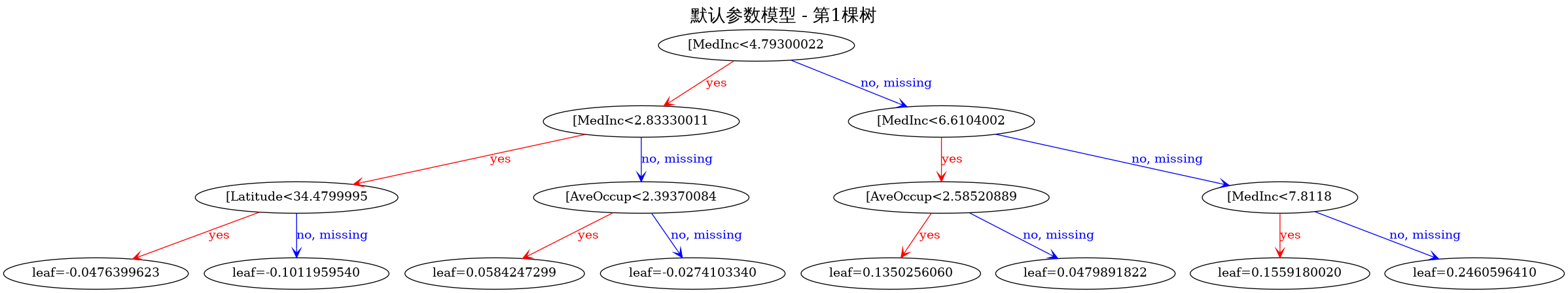
        # 绘制默认参数模型的第一棵树
        plot_tree(default_model, 
                  num_trees=0,  # 第一棵树
                  ax=ax1,
                  rankdir='TB',
                  max_depth=3)  # 限制显示深度以保证可读性
        ax1.set_title('XGBoost 树结构 - 默认参数 (第1棵树)', fontsize=14, fontweight='bold')
        
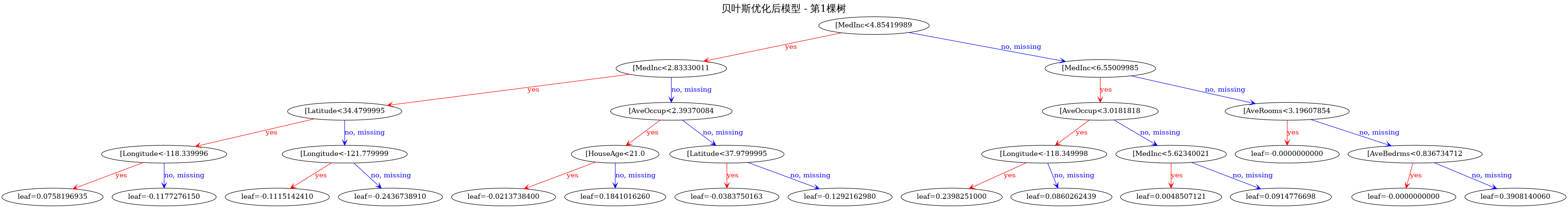
        # 绘制优化后模型的第一棵树
        plot_tree(best_model, 
                  num_trees=0,  # 第一棵树
                  ax=ax2,
                  rankdir='TB',
                  max_depth=3)  # 限制显示深度以保证可读性
        ax2.set_title('XGBoost 树结构 - 贝叶斯优化后 (第1棵树)', fontsize=14, fontweight='bold')
        
        plt.tight_layout()
        plt.savefig('xgboost_tree_comparison.png', dpi=300, bbox_inches='tight')
        plt.show()
        
        print("树结构对比图已保存为'xgboost_tree_comparison.png'")
        
        # 额外生成详细的树结构信息对比
        print("\n树结构参数对比:")
        print("=" * 50)
        print("默认参数模型:")
        print(f"  树的数量: {default_model.n_estimators}")
        print(f"  最大深度: {default_model.max_depth}")
        print(f"  学习率: {default_model.learning_rate}")
        print(f"  子样本比例: {default_model.subsample}")
        print(f"  特征子样本比例: {default_model.colsample_bytree}")
        
        print("\n贝叶斯优化后模型:")
        print(f"  树的数量: {best_model.n_estimators}")
        print(f"  最大深度: {best_model.max_depth}")
        print(f"  学习率: {best_model.learning_rate}")
        print(f"  子样本比例: {best_model.subsample}")
        print(f"  特征子样本比例: {best_model.colsample_bytree}")
        print(f"  L1正则化: {best_model.reg_alpha}")
        print(f"  L2正则化: {best_model.reg_lambda}")
        
        # 生成多棵树的对比（如果需要更详细的分析）
        print("\n生成前3棵树的详细对比...")
        fig, axes = plt.subplots(2, 3, figsize=(24, 16))
        
        for i in range(3):
            # 默认参数模型的树
            plot_tree(default_model, 
                      num_trees=i,
                      ax=axes[0, i],
                      rankdir='TB',
                      max_depth=2)  # 进一步限制深度以保证可读性
            axes[0, i].set_title(f'默认参数 - 第{i+1}棵树', fontsize=12)
            
            # 优化后模型的树
            plot_tree(best_model, 
                      num_trees=i,
                      ax=axes[1, i],
                      rankdir='TB',
                      max_depth=2)  # 进一步限制深度以保证可读性
            axes[1, i].set_title(f'贝叶斯优化后 - 第{i+1}棵树', fontsize=12)
        
        plt.suptitle('XGBoost 前3棵树结构对比', fontsize=16, fontweight='bold')
        plt.tight_layout()
        plt.savefig('xgboost_multiple_trees_comparison.png', dpi=300, bbox_inches='tight')
        plt.show()
        
        print("多棵树对比图已保存为'xgboost_multiple_trees_comparison.png'")

    except ImportError:
        print("注意: 需要安装graphviz来显示树结构图")
        print("可以通过以下命令安装:")
        print("pip install graphviz")
        print("或者: conda install graphviz")
        
        # 备选方案：生成树结构统计信息对比
        print("\n使用文本形式展示树结构对比信息:")
        print("=" * 50)
        
        # 获取树的统计信息
        def get_tree_stats(model):
            booster = model.get_booster()
            tree_df = booster.trees_to_dataframe()
            stats = {
                'total_nodes': len(tree_df),
                'leaf_nodes': len(tree_df[tree_df['Feature'] == 'Leaf']),
                'split_nodes': len(tree_df[tree_df['Feature'] != 'Leaf']),
                'avg_depth': tree_df.groupby('Tree')['Node'].count().mean(),
                'max_depth': tree_df.groupby('Tree')['Node'].count().max()
            }
            return stats
        
        default_stats = get_tree_stats(default_model)
        optimized_stats = get_tree_stats(best_model)
        
        print("默认参数模型树结构统计:")
        for key, value in default_stats.items():
            print(f"  {key}: {value:.2f}")
        
        print("\n贝叶斯优化后模型树结构统计:")
        for key, value in optimized_stats.items():
            print(f"  {key}: {value:.2f}")

    except Exception as e:
        print(f"生成树结构图时出现错误: {e}")
        print("将继续执行其他部分...")

    # 保存最优参数到文件
    with open('best_params.txt', 'w', encoding='utf-8') as f:
        f.write("XGBoost 贝叶斯优化最佳参数:\n")
        f.write("=" * 40 + "\n")
        for param, value in bayes_search.best_params_.items():
            f.write(f"{param}: {value}\n")
        f.write(f"\n最佳CV分数: {-bayes_search.best_score_:.4f}\n")
        f.write(f"测试集RMSE: {rmse:.4f}\n")
        f.write(f"测试集R²: {r2:.4f}\n")
        f.write(f"优化耗时: {optimization_time:.2f} 秒\n")

    print("最优参数已保存到'best_params.txt'")

except KeyboardInterrupt:
    print("\n用户中断了优化过程")
except Exception as e:
    print(f"\n优化过程中出现错误: {e}")
    print("建议进一步减少参数范围或数据集大小")

print("\n程序执行完成！")

最后的运行结果如下: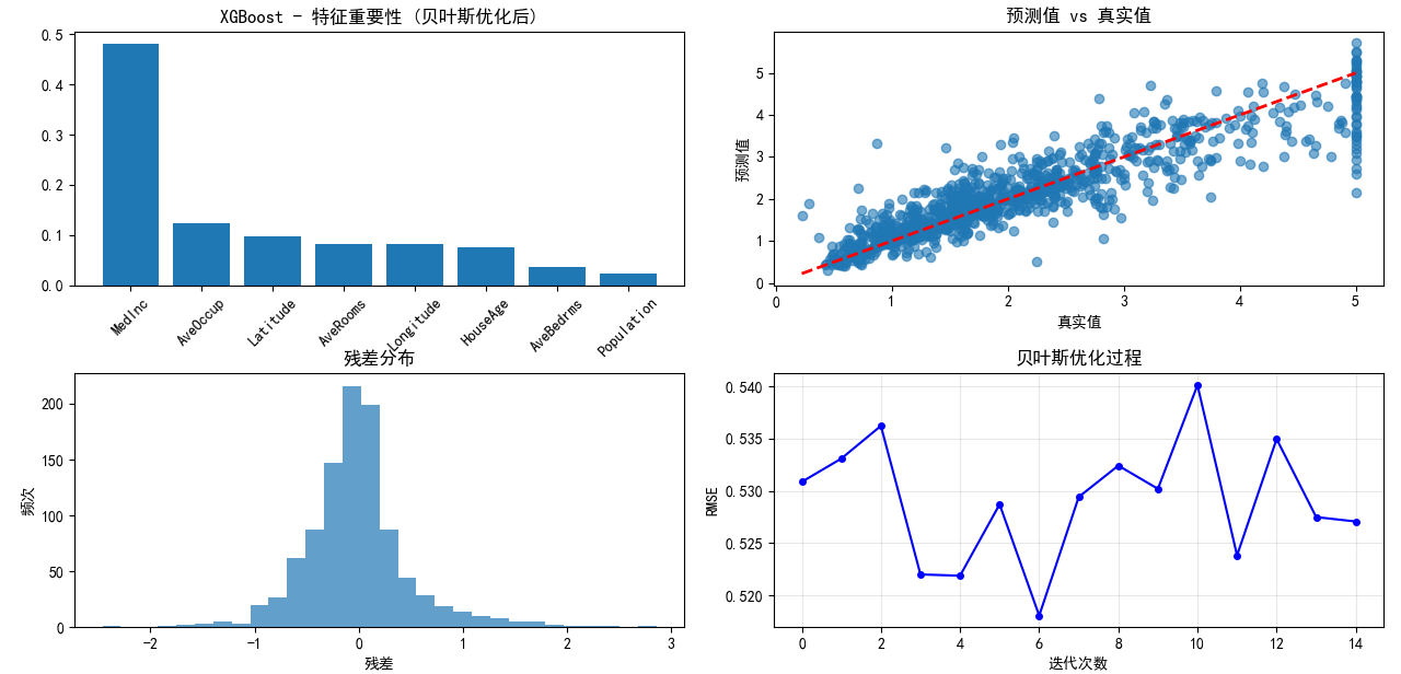

可以看到在贝叶斯参数的前后，XGboost的准确性发生了巨大的变化，RMSE和R{^2}分别改善了7.24%和3.97%。这反映了贝叶斯参数优化的可行性和高效性。

XGboost在回归分析中的使用

Xgboost除了应用于二分类以外，还可以用于回归和拟合，他们在数学原理上并不完全相同，但存在着相似之处:

二分类:

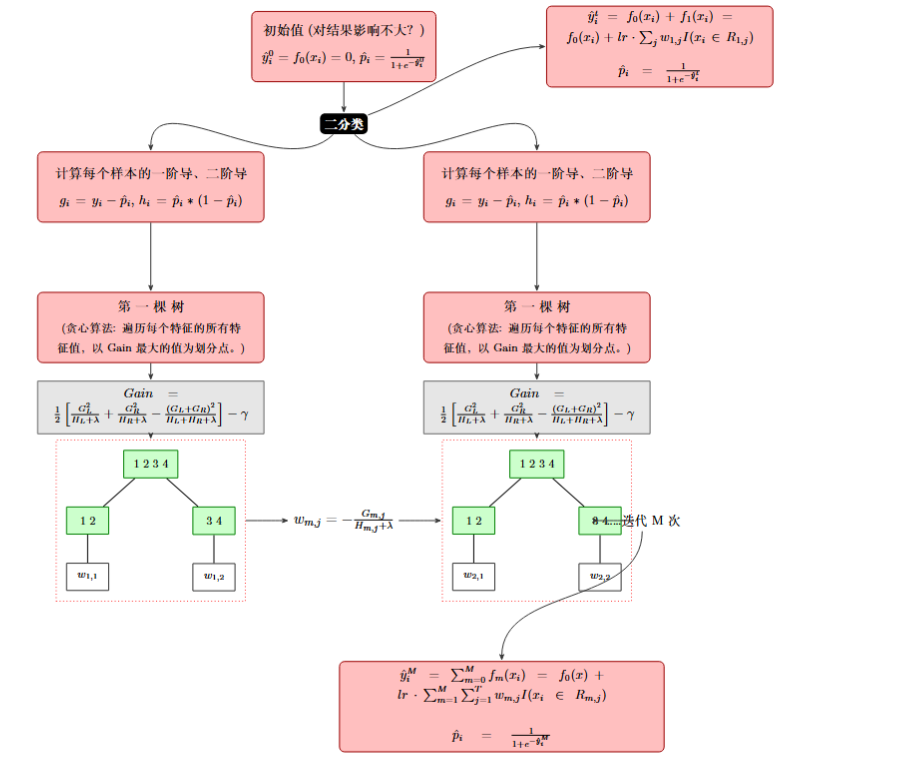
回归: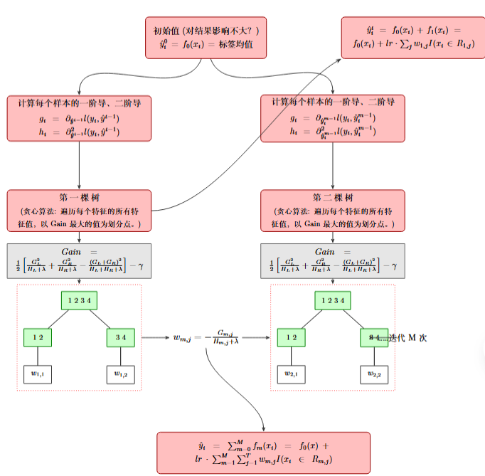

同样用相同的股市进行使用XGboost进行回归和拟合，其相应的代码如下:

import xgboost as xgb
import pandas as pd
import numpy as np
from sklearn.datasets import fetch_california_housing
from sklearn.model_selection import train_test_split
from sklearn.metrics import mean_squared_error, r2_score
import matplotlib.pyplot as plt
import seaborn as sns

plt.rcParams['font.sans-serif'] = ['SimHei', 'Microsoft YaHei', 'Arial Unicode MS']
plt.rcParams['axes.unicode_minus'] = False


print(f"XGBoost version: {xgb.__version__}")

# 2. 加载并了解数据集
housing = fetch_california_housing()
X, y = housing.data, housing.target
df = pd.DataFrame(X, columns=housing.feature_names)
df['MedHouseVal'] = y
print("数据集前5行:")
print(df.head())
print("\n数据集特征:")
print(housing.feature_names)
print("\n数据集目标 (需要预测的值):")
print("MedHouseVal (房屋价值中位数)")

# 3. 数据准备
X_train, X_test, y_train, y_test = train_test_split(X, y, test_size=0.2, random_state=42)
print(f"\n训练集大小: {X_train.shape}")
print(f"测试集大小: {X_test.shape}")

# 4. 创建并训练XGBoost回归模型
xg_reg = xgb.XGBRegressor(objective='reg:squarederror', 
                          n_estimators=1000, 
                          learning_rate=0.05,
                          max_depth=5,
                          subsample=0.8,
                          colsample_bytree=0.8,
                          random_state=42,
                          n_jobs=-1)

print("\n开始训练XGBoost模型...")

# XGBoost 3.0+ 版本的训练
xg_reg.fit(X_train, y_train, 
           eval_set=[(X_test, y_test)], 
           verbose=False)

print("模型训练完成。")

# 5. 在测试集上进行预测
y_pred = xg_reg.predict(X_test)

# 6. 评估模型性能
rmse = np.sqrt(mean_squared_error(y_test, y_pred))
r2 = r2_score(y_test, y_pred)
print(f"\n模型性能评估:")
print(f"均方根误差 (RMSE): {rmse:.4f}")
print(f"R² 分数 (R-squared): {r2:.4f}")
if hasattr(xg_reg, 'best_iteration') and xg_reg.best_iteration:
    print(f"模型在第 {xg_reg.best_iteration} 轮迭代时效果最佳。")

# 7. 特征重要性可视化
try:
    feature_importance = xg_reg.feature_importances_
    feature_names = housing.feature_names

    # 创建特征重要性图
    indices = np.argsort(feature_importance)[::-1]
    plt.figure(figsize=(12, 8))
    plt.title('XGBoost 特征重要性分析', fontsize=16, fontweight='bold')
    plt.bar(range(len(feature_importance)), feature_importance[indices])
    plt.xticks(range(len(feature_importance)), [feature_names[i] for i in indices], rotation=45)
    plt.xlabel('特征名称', fontsize=12)
    plt.ylabel('重要性得分', fontsize=12)
    plt.tight_layout()
    plt.show()
    print("特征重要性图表显示成功")
except Exception as e:
    print(f"特征重要性可视化异常: {e}")
    import traceback
    traceback.print_exc()

# 8. 真实值 vs 预测值 可视化
try:
    plt.figure(figsize=(10, 10))
    plt.scatter(y_test, y_pred, alpha=0.3, color='blue', s=20)
    plt.plot([y_test.min(), y_test.max()], [y_test.min(), y_test.max()], '--r', linewidth=2, label='完美预测线')
    plt.xlabel('实际房价值（万美元）', fontsize=12)
    plt.ylabel('预测房价值（万美元）', fontsize=12)
    plt.title('加州房价预测模型：实际值 vs 预测值对比', fontsize=14, fontweight='bold')
    plt.legend()
    plt.grid(True, alpha=0.3)
    plt.axis('equal')
    plt.axis('square')

    # 添加R²分数到图表上 - 修复显示问题
    plt.text(0.05, 0.95, f'R-squared = {r2:.4f}\nRMSE = {rmse:.4f}', 
             transform=plt.gca().transAxes, fontsize=12,
             verticalalignment='top', bbox=dict(boxstyle='round', facecolor='wheat', alpha=0.8))
    plt.tight_layout()
    plt.show()
    print("预测对比图表显示成功")
except Exception as e:
    print(f"预测对比可视化异常: {e}")
    import traceback
    traceback.print_exc()

print("程序执行完毕")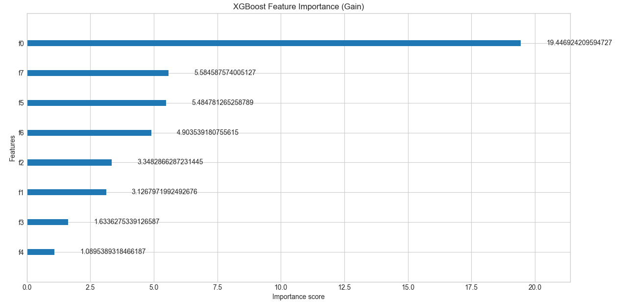

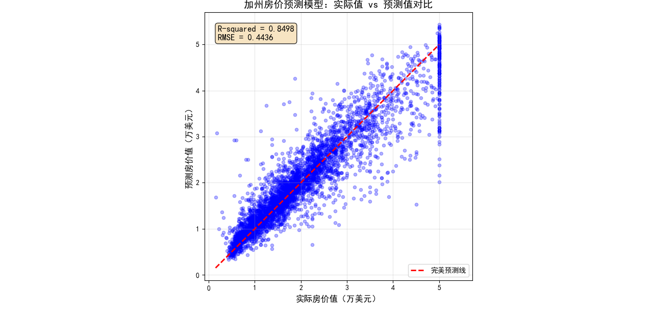
得到最后的结果如上所示。