MOP问题
多目标规划问题,一般来说存在多个优化函数即可称为多目标规划问题,解决这一问题有一种常用的解法:确定不同函数的权重,然后构造一个新的函数,通过对这个函数使用优化算法从而得到结果。这种方法实际上解决的仍然是单目标的规划问题,因为其仅对单函数进行分析。然而NSGA-II算法则是基于帕累托最优利用非支配排序解决多目标规划问题的利器。
Pareto图
Pareto原则就是为人熟知的“二八法则,”即多数的资源在少数人的手中。利用这一规则也可以间接地判断某一优化方向与众多变量之间的累积贡献率,利用pareto原则可以达到降维的目的。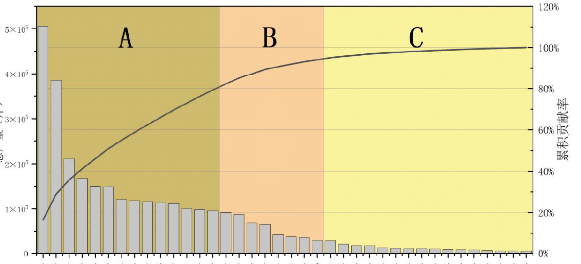
pareto图直观地反映了变量的积累效应,与PCA的原理类似。
Pareto前沿
Pareto前沿指的是当多个方向的优化都达到最优情况下各点所连成的曲线(在双目标规划问题的情况下是二维曲线,三目标规划问题则是三维的曲面)。
举一个生活中的例子,如果一个商务客服在工作方面投入时间与遭投诉次数之间的联系:前者较大时,后者必然较小,反之则规律相反。如果我们在图中以二维的形式画出这张图便有如下的形式: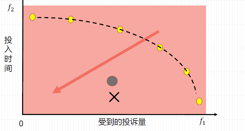
而对于Pareto前沿上的各点,其之间是不存在优劣区别的。这也正是NGSA-II算法所需要利用的地方。
非支配排序
支配与非支配的概念
支配排序指的是可以严格判断A点和B点的优劣,例如下图所示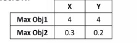
如果X和Y的第一指标最大值都是4,然而X的第二指标最大值时大于Y的,那么可以认为X是严格优于Y的。这种情况一般被称为支配排序。而对于非支配排序则是像下面这种,无法严格判断他们的优劣: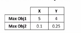
因此对于非支配排序实际上是我们所需要深入研究的,因为支配排序的比较是非常简单的。非支配排序主流的方法是拥挤距离法。
拥挤距离
拥挤距离的计算与曼哈顿距离的计算是类似的,都是绝对值距离。在如下的图中:
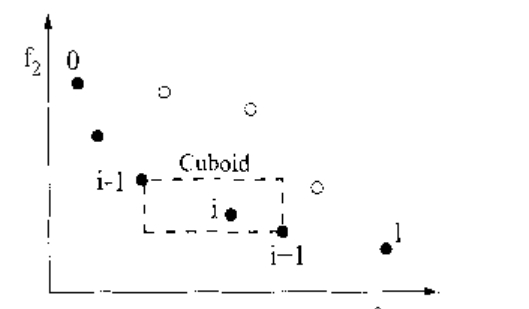
点i的拥挤度与i-1和i+1是相关的,我们可以构造以i-1 和i+1 所围成的矩形以其周长表述它的拥挤度。NSGA-II原文献中对拥挤度的定义如下: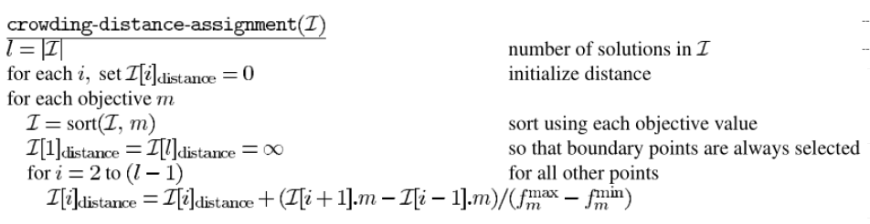
需要注意的是我们一般取拥挤度大的地方作为Pareto前沿,这是因为拥挤度大的话可以避免种群之间的相互影响,以提高物种多样性(类似于禁止近亲结婚,以提高人群精英)
非支配排序利用拥挤距离评判大小!!!
遗传算法与pareto前沿的结合
算法的流程:
初始化N 个解个体
计算函数值 或者适应度
利用旧解产生新解
各种策略: GA, PSO , 灰狼优化等 本质一样
选择得到新一轮的解
利用支配排序和非支配排序的拥挤距离进行解的判断
遗传算法的几个常见操作:
1.交叉
即交配,假设前一代是x_1和x_2,那么子代有可能得到前一代的全部优良性状,生成0.5(x_1+x_2),
然后将0.5(x_1+x_2) 所对应的适应度函数与父代中的x_1 和x_2 进行排序,判断是否需要取此点。
2.变异
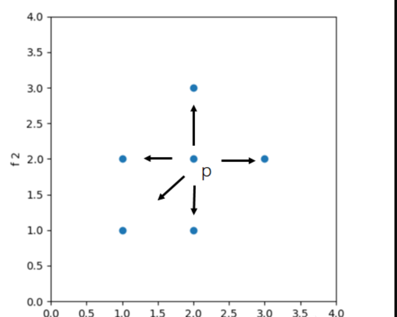
如图所示,任一点P都有着朝四个方向进行变异的可能性,且变化是随机的,例如使其加上0.1或减去0.2。接着继续计算适应度函数以确定是否需要把变异的结果保留,从而提高了多样性。
经过上述的分析和图像的特征,我们可以发现越是靠近坐标左下角的点就越是有可能是pareto前沿上的点。因此越靠近左下越好!!!
NSGA代码分析
根据以上信息,我们确定了适应度函数之后需要先进行取点,随后进行遗传的各项操作,(利用二进制转码实现),然后判断排序,随后即可绘制pareto图,并求出极值。
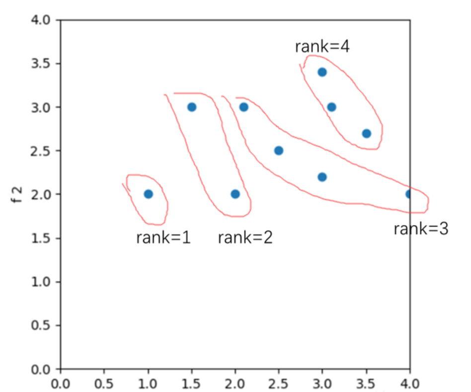
排序的时候,很明显我们可以得到如图的第一、第二、第三梯队。
NSGA-I
关键步骤排序的伪代码如下:
Pop = pop
i = 1

while Pop:
    for pi in Pop:
        pi.dominatecount = 0
        for pj in Pop:
            if pj < pi:
                pi.dominatecount += 1

    S = [pi for pi in Pop if pi.dominatecount == 0]

    for pi in S:
        pi.Rank = i  # 标记这是第几层

    F.append(S)      # 记录每一层的个体
    Pop = Pop - set(S)  # 下一轮两两比较
    i += 1
可以注意到其最严重的时间复杂度是O(Mn^3)
其求解的过程是复杂的,因此这也是NSGA-I被NSGA-II所淘汰的原因
NSGA-II
依据以上分析NSGA-II的伪代码如下
def fast_non_dominated_sort(P):
    S = {}          # 存储每个个体 p 所支配的个体集合
    n = {}          # 存储每个个体 p 被支配的个数
    rank = {}       # 存储每个个体的等级
    F = [[]]        # 第一层前沿

    for p in P:
        S[p] = []
        n[p] = 0
        for q in P:
            if p ≺ q:                      # p dominates q
                S[p].append(q)
            elif q ≺ p:                    # q dominates p
                n[p] += 1
        if n[p] == 0:
            rank[p] = 1
            F[0].append(p)

    i = 0
    while F[i]:
        Q = []
        for p in F[i]:
            for q in S[p]:
                n[q] -= 1
                if n[q] == 0:
                    rank[q] = i + 2
                    Q.append(q)
        i += 1
        F.append(Q)

    return F
同样是两两比较,但第II代NSGA使用了更好的数据结构:
S[p]记录 p 支配了谁。n[p]记录 p 被多少人支配。
因此NSGA-II的最坏计算复杂度仅为O(MN^2)
计算的速度和时间更快,收敛性更强,这也正是NSGA-II算法得到广泛应用的原因。
NSGA-II Matlab实现
这里以ZDT1测试函数为例,其NSGA-II实现的matlab代码如下:
%% 主函数:NSGA-II 多目标优化算法
function nsga_2_optimization
% 可修改参数区
pop = 200;    % 种群数量
gen = 500;    % 迭代次数
M = 2;        % 目标函数数量
V = 30;       % 维度(决策变量的个数)
min_range = zeros(1, V); % 下界 生成1*30的个体向量 全为0
max_range = ones(1,V);   % 上界 生成1*30的个体向量 全为1

% 初始化种群
chromosome = initialize_variables(pop, M, V, min_range, max_range);
chromosome = non_domination_sort_mod(chromosome, M, V);

% 主循环
for i = 1 : gen
    pool = round(pop/2);
    tour = 2;

    parent_chromosome = tournament_selection(chromosome, pool, tour);

    mu = 20;
    mum = 20;

    offspring_chromosome = genetic_operator(parent_chromosome, M, V, mu, mum, min_range, max_range);

    [main_pop, ~] = size(chromosome);
    [offspring_pop, ~] = size(offspring_chromosome);

    clear temp
    intermediate_chromosome(1:main_pop,:) = chromosome;
    intermediate_chromosome(main_pop + 1 : main_pop + offspring_pop, 1 : M+V) = offspring_chromosome;

    intermediate_chromosome = non_domination_sort_mod(intermediate_chromosome, M, V);

    chromosome = replace_chromosome(intermediate_chromosome, M, V, pop);

    if ~mod(i,100)
        clc;
        fprintf('%d generations completed\n', i);
    end
end

% 绘制帕累托前沿
if M == 2
    plot(chromosome(:,V + 1), chromosome(:,V + 2), '*');
    xlabel('f_1'); ylabel('f_2');
    title('Pareto Optimal Front');
elseif M == 3
    plot3(chromosome(:,V + 1), chromosome(:,V + 2), chromosome(:,V + 3), '*');
    xlabel('f_1'); ylabel('f_2'); zlabel('f_3');
    title('Pareto Optimal Surface');
end
end

%% 目标函数评价 - 计算每个个体的目标函数值
function f = evaluate_objective(x, M, V)
f = [];
f(1) = x(1);
g = 1;
sum = 0;
for i = 2:V
    sum = sum + x(i);
end
sum = 9*(sum / (V-1));
g = g + sum;
f(2) = g * (1 - sqrt(x(1) / g));
end

%% 初始化种群
function f = initialize_variables(N, M, V, min_range, max_range)
min = min_range;
max = max_range;
K = M + V;
for i = 1 : N
    for j = 1 : V
        f(i,j) = min(j) + (max(j) - min(j))*rand(1);
    end
    f(i,V + 1: K) = evaluate_objective(f(i,:), M, V);
end
end

%% 非支配排序和拥挤度计算
function f = non_domination_sort_mod(x, M, V)
[N, ~] = size(x);
clear m
front = 1;
F(front).f = [];
individual = [];

for i = 1 : N
    individual(i).n = 0;
    individual(i).p = [];
    for j = 1 : N
        dom_less = 0;
        dom_equal = 0;
        dom_more = 0;
        for k = 1 : M
            if (x(i,V + k) < x(j,V + k))
                dom_less = dom_less + 1;
            elseif (x(i,V + k) == x(j,V + k))
                dom_equal = dom_equal + 1;
            else
                dom_more = dom_more + 1;
            end
        end
        if dom_less == 0 && dom_equal ~= M
            individual(i).n = individual(i).n + 1;
        elseif dom_more == 0 && dom_equal ~= M
            individual(i).p = [individual(i).p j];
        end
    end
    if individual(i).n == 0
        x(i,M + V + 1) = 1;
        F(front).f = [F(front).f i];
    end
end

while ~isempty(F(front).f)
   Q = [];
   for i = 1 : length(F(front).f)
       if ~isempty(individual(F(front).f(i)).p)
            for j = 1 : length(individual(F(front).f(i)).p)
                individual(individual(F(front).f(i)).p(j)).n = ...
                    individual(individual(F(front).f(i)).p(j)).n - 1;
                    if individual(individual(F(front).f(i)).p(j)).n == 0
                       x(individual(F(front).f(i)).p(j), M + V + 1) = ...
                        front + 1;
                    Q = [Q individual(F(front).f(i)).p(j)];
                end
            end
       end
   end
   front = front + 1;
   F(front).f = Q;
end

[~, index_of_fronts] = sort(x(:,M + V + 1));
sorted_based_on_front = x(index_of_fronts,:);
current_index = 0;

for front = 1 : (length(F) - 1)
    distance = 0;
    y = [];
    previous_index = current_index + 1;
    for i = 1 : length(F(front).f)
        y(i,:) = sorted_based_on_front(current_index + i,:);
    end
    current_index = current_index + i;
    sorted_based_on_objective = [];
    for i = 1 : M
        [~, index_of_objectives] = sort(y(:,V + i));
        sorted_based_on_objective = [];
        for j = 1 : length(index_of_objectives)
            sorted_based_on_objective(j,:) = y(index_of_objectives(j),:);
        end
        f_max = sorted_based_on_objective(length(index_of_objectives), V + i);
        f_min = sorted_based_on_objective(1, V + i);

        y(index_of_objectives(length(index_of_objectives)), M + V + 1 + i) = Inf;
        y(index_of_objectives(1), M + V + 1 + i) = Inf;

        for j = 2 : length(index_of_objectives) - 1
            next_obj = sorted_based_on_objective(j + 1, V + i);
            previous_obj = sorted_based_on_objective(j - 1, V + i);
            if (f_max - f_min == 0)
                y(index_of_objectives(j), M + V + 1 + i) = Inf;
            else
                y(index_of_objectives(j), M + V + 1 + i) = (next_obj - previous_obj)/(f_max - f_min);
            end
        end
    end

    distance = [];
    distance(:,1) = zeros(length(F(front).f), 1);
    for i = 1 : M
        distance(:,1) = distance(:,1) + y(:,M + V + 1 + i);
    end
    y(:,M + V + 2) = distance;
    y = y(:,1 : M + V + 2);
    z(previous_index:current_index,:) = y;
end
f = z();
end

%% 锦标赛选择
function f = tournament_selection(chromosome, pool_size, tour_size)
[pop, variables] = size(chromosome);
rank = variables - 1;
distance = variables;

for i = 1 : pool_size
    for j = 1 : tour_size
        candidate(j) = round(pop*rand(1));
        if candidate(j) == 0
            candidate(j) = 1;
        end
        if j > 1
            while ~isempty(find(candidate(1 : j - 1) == candidate(j)))
                candidate(j) = round(pop*rand(1));
                if candidate(j) == 0
                    candidate(j) = 1;
                end
            end
        end
    end

    for j = 1 : tour_size
        c_obj_rank(j) = chromosome(candidate(j), rank);
        c_obj_distance(j) = chromosome(candidate(j), distance);
    end

    min_candidate = find(c_obj_rank == min(c_obj_rank));
    if length(min_candidate) ~= 1
        max_candidate = find(c_obj_distance(min_candidate) == max(c_obj_distance(min_candidate)));
        if length(max_candidate) ~= 1
            max_candidate = max_candidate(1);
        end
        f(i,:) = chromosome(candidate(min_candidate(max_candidate)),:);
    else
        f(i,:) = chromosome(candidate(min_candidate(1)),:);
    end
end
end

%% 遗传算子
function f = genetic_operator(parent_chromosome, M, V, mu, mum, l_limit, u_limit)
[N, ~] = size(parent_chromosome);

p = 1;
was_crossover = 0;
was_mutation = 0;

for i = 1 : N
    if rand(1) < 0.9
        child_1 = [];
        child_2 = [];

        parent_1 = round(N*rand(1));
        if parent_1 < 1
            parent_1 = 1;
        end
        parent_2 = round(N*rand(1));
        if parent_2 < 1
            parent_2 = 1;
        end
        while isequal(parent_chromosome(parent_1,:), parent_chromosome(parent_2,:))
            parent_2 = round(N*rand(1));
            if parent_2 < 1
                parent_2 = 1;
            end
        end
        parent_1 = parent_chromosome(parent_1,:);
        parent_2 = parent_chromosome(parent_2,:);

        for j = 1 : V
            u(j) = rand(1);
            if u(j) <= 0.5
                bq(j) = (2*u(j))^(1/(mu+1));
            else
                bq(j) = (1/(2*(1 - u(j))))^(1/(mu+1));
            end
            child_1(j) = 0.5*(((1 + bq(j))*parent_1(j)) + (1 - bq(j))*parent_2(j));
            child_2(j) = 0.5*(((1 - bq(j))*parent_1(j)) + (1 + bq(j))*parent_2(j));

            if child_1(j) > u_limit(j)
                child_1(j) = u_limit(j);
            elseif child_1(j) < l_limit(j)
                child_1(j) = l_limit(j);
            end
            if child_2(j) > u_limit(j)
                child_2(j) = u_limit(j);
            elseif child_2(j) < l_limit(j)
                child_2(j) = l_limit(j);
            end
        end

        child_1(:,V + 1: M + V) = evaluate_objective(child_1, M, V);
        child_2(:,V + 1: M + V) = evaluate_objective(child_2, M, V);

        was_crossover = 1;
        was_mutation = 0;
    else
        parent_3 = round(N*rand(1));
        if parent_3 < 1
            parent_3 = 1;
        end
        child_3 = parent_chromosome(parent_3,:);

        for j = 1 : V
           r(j) = rand(1);
           if r(j) < 0.5
               delta(j) = (2*r(j))^(1/(mum+1)) - 1;
           else
               delta(j) = 1 - (2*(1 - r(j)))^(1/(mum+1));
           end
           child_3(j) = child_3(j) + delta(j);

           if child_3(j) > u_limit(j)
               child_3(j) = u_limit(j);
           elseif child_3(j) < l_limit(j)
               child_3(j) = l_limit(j);
           end
        end

        child_3(:,V + 1: M + V) = evaluate_objective(child_3, M, V);

        was_mutation = 1;
        was_crossover = 0;
    end

    if was_crossover
        child(p,:) = child_1;
        child(p+1,:) = child_2;
        was_crossover = 0;
        p = p + 2;
    elseif was_mutation
        child(p,:) = child_3(1,1 : M + V);
        was_mutation = 0;
        p = p + 1;
    end
end

f = child;
end

%% 精英选择策略
function f = replace_chromosome(intermediate_chromosome, M, V, pop)
[N, ~] = size(intermediate_chromosome);
[~, index] = sort(intermediate_chromosome(:, M + V + 1));

for i = 1 : N
    sorted_chromosome(i,:) = intermediate_chromosome(index(i),:);
end

max_rank = max(intermediate_chromosome(:, M + V + 1));

previous_index = 0;
for i = 1 : max_rank
    current_index = max(find(sorted_chromosome(:, M + V + 1) == i));
    if current_index > pop
        remaining = pop - previous_index;
        temp_pop = sorted_chromosome(previous_index + 1 : current_index, :);

        [~, temp_sort_index] = sort(temp_pop(:, M + V + 2), 'descend');
        for j = 1 : remaining
            f(previous_index + j,:) = temp_pop(temp_sort_index(j),:);
        end
        return;
    elseif current_index < pop
        f(previous_index + 1 : current_index, :) = sorted_chromosome(previous_index + 1 : current_index, :);
    else
        f(previous_index + 1 : current_index, :) = sorted_chromosome(previous_index + 1 : current_index, :);
        return;
    end
    previous_index = current_index;
end
end
在运行之后我们可以得到如下的结果:
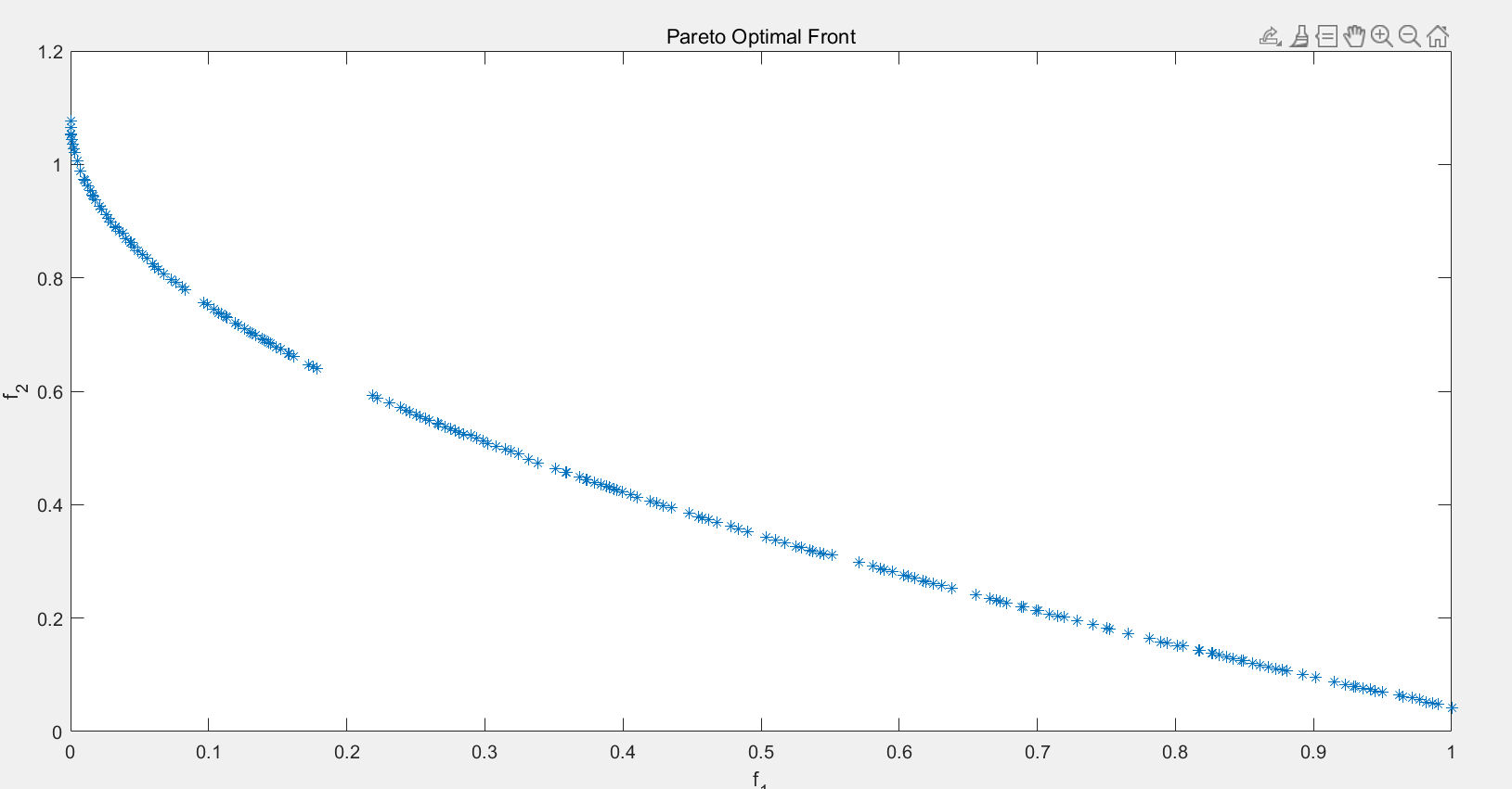
其中蓝线正是pareto前沿,即最佳取值的各指标优化方向。
总结
NSGA-II以其收敛快、多样性好、鲁棒性强、计算效率高同时拥挤距离保多样性,精英保留加速收敛而成为了解决MOP问题的优秀智能启发式算法。