Missing aircraft search and rescue model based on diverse actual open water situations
Summary
Maritime search and rescue (SAR) is a vital task, however, traditional methods have
many limitations, so it is imperative to optimise search and rescue methods. This can not
only improve the success rate of SAR and save more lives, but also save a lot of manpower,
material and time costs and enhance the maritime emergency rescue capability. Therefore,
we established a general model for predicting the possible crash area of an aircraft after
crashing at sea and used software to derive a crash probability density distribution map,
using Monte Carlo model simulation and annealing algorithm to optimize the search and
rescue strategy. We divided the whole project into three sub-tasks.
In Task 1: Considering factors such as aircraft disintegration in the air, air density
change with altitude, lateral wind, etc., we divided the whole crash process into two
parts, before and after entering water. We initially established the physical model of the
aircraft losing power from the normal flight altitude and crashing, set up the mechanical
equations, and solved them using MATLAB.
In Task 2: We introduced the concept of the aircraft steering slope angle, calculated
its trajectory, and finally calculated its final possible crash range by adjusting the param-
eter range, analogous to the Galton plate model, plotted the probability density of the
aircraft’s probability density function of the possible landing points, divided into several
blocks, and obtained the probability density of crashing in any one of these areas, and
then obtained the total probability density.
In Task 3: As we know, there are two main directions for the optimisation of the rescue
operation: to make the probability of rescuing the crash victims large, and to make rescue
time small. Therefore, we propose two methods to achieve the optimisation.
Method 1 : The spiral search and rescue model
Method 2 : The Monte Carlo simulation-traveler search and rescue model
In the sensitivity analysis section.,the assumptions we made in task 1 to simplify the
model are as follows:
Not considering the disintegration of the aircraft in the air.
Not considering the change of air density with altitude.
Not considering the effect of lateral winds.
Consider them separately to optimize the previous model to make it more reasonable,
more practical, and more applicable.
Keywords: normal distribution, binary normal distribution, Monte Carlo simulation,
simulated annealing algorithm
Contents
1 Introduction
2 Issue Restated
3 Assumptions and Justifications
4 Analysis of the Problem
5 Notations
6 Task 1: Physical modeling of aircraft crashes
7 Task 2: The representation of the probability density
8 Task 3: Optimization of Search and Rescue Strategies
8.1 Strategy 1: Spiral Search and Rescue Model
8.2 Strategy 2: Monte Carlo simulation-traveler search and rescue model
9 Sensitivity analysis
9.1 Analysis of the effects of ocean currents
9.2 Analysis of the effects of changes in air density with altitude
9.3 Analysis of the effects of lateral wind effects
10 Conclusions
11 Strengths and weaknesses
11.1 Strengths
11.2 Weeknesses
12 References
Appendices
1 Introduction
The accident of Malaysia Airlines MH370 is heartbreaking, part of the remains have not
been found yet, and most of the existing SAR models are based on Bayesian statistical
methods. To better enhance the segmentation properties of the SAR model, we establish a
mathematical model and a search and rescue plan for maritime SAR, aiming to efficiently
carry out SAR work in the shortest possible time, and practically safeguard the safety of
lives and save losses.
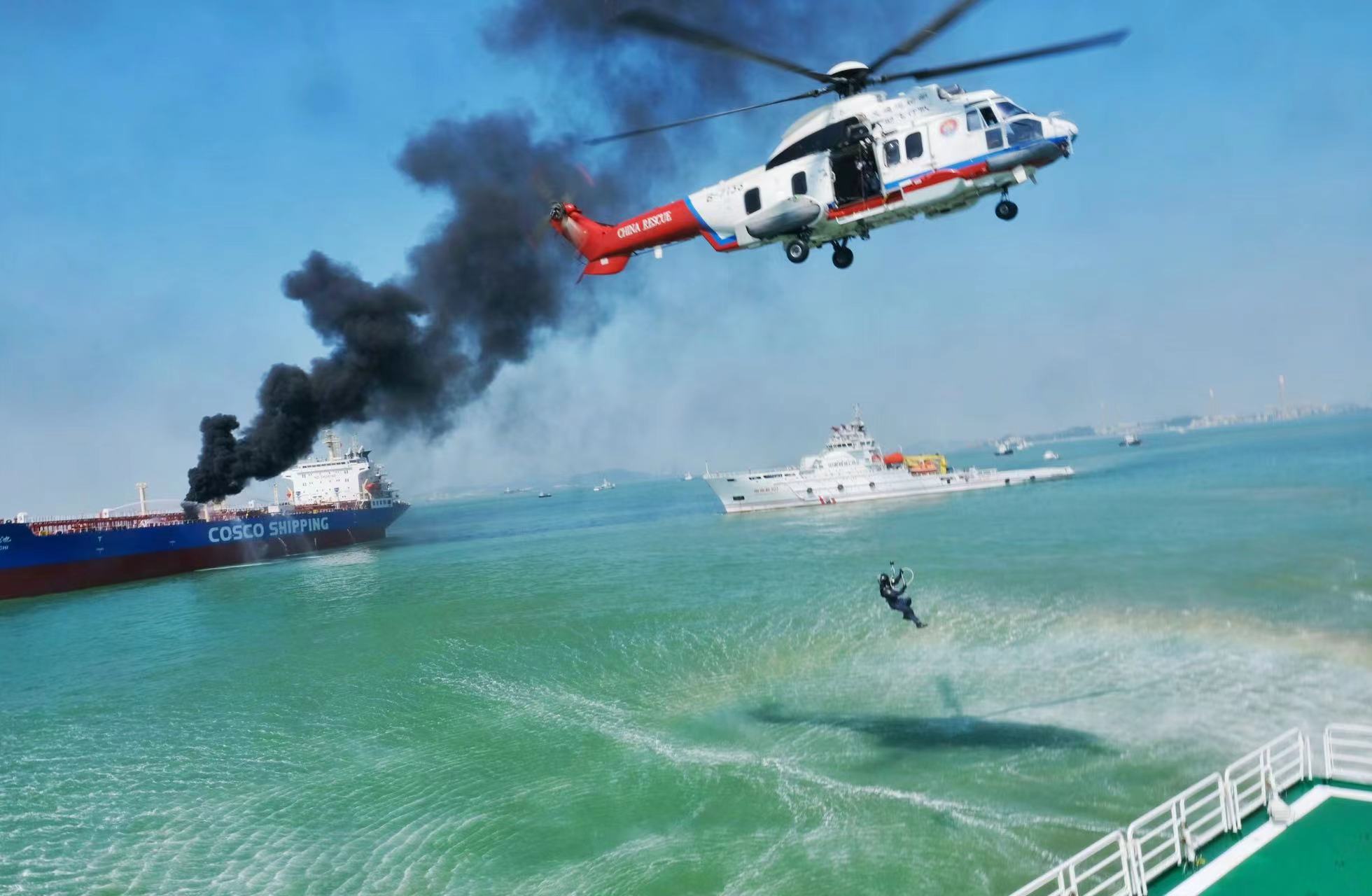
Figure 1: Simulated maritime search and rescue operations
2 Issue Restated
On March 8, 2014, Malaysia Airlines flight 370 from Kuala Lumpur to Beijing took off from Kuala Lumpur International Airport at 0:41 a.m. Malaysian Standard Time (MST) with 239 people on board. The flight was scheduled to arrive at Beijing Capital Interna- tional Airport at 6:30 a.m. Beijing time, but less than an hour after takeoff, it lost contact with Malaysia’s Subang Air Traffic Control Center (SATC) at the Malaysian-Vietnamese sea border, about 140 nautical miles south of Tuju Island and about 90 nautical miles east- northeast of Kota Bharu. After the crash, the community mobilized a large number of search and rescue teams and supplies to rescue the aircraft, but so far there is still no result, and the incident finally ended with the loss of the aircraft. In the aftermath of a plane crash, it is crucial to construct a reasonable model to determine the possible crash site of the crashed plane and the arrangement of rescue teams to conduct the search and rescue program, as they will directly affect the efficiency and success rate of the search and rescue process.
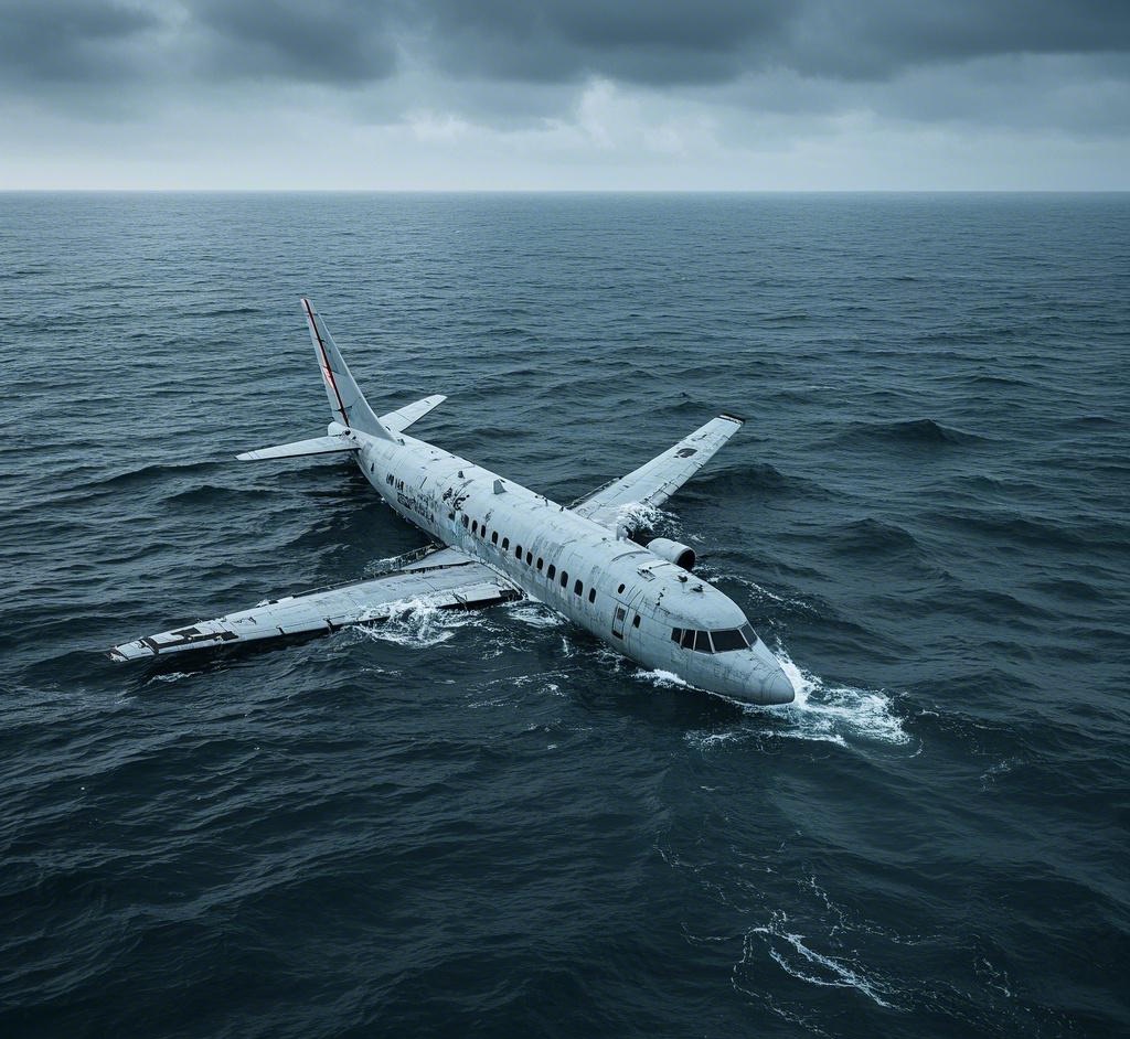
Figure 2: Schematic of the airplane crash site
3 Assumptions and Justifications
- Assumption 1 : The airplane was not hijacked and the crash was due to a failure of the airplane’s power system.
- Justification 1 :Consideration of relevant technicalities only.
- Assumption 2 : There were no physical changes in the airplane during the crash, and the mass, volume, area, etc. did not change.
- Justification 2 : Discussion of the disintegrated pieces of an airplane will only add to the uncertainty since they are subjected to similar forces due to their inertial velocity being the same as the main part.
4 Analysis of the Problem
The problem requires the establishment of a general mathematical model for planning search operations for missing aircraft in open waters (such as oceans) under signal-less conditions. This model must be adaptable to various types of aircraft and differences in
search equipment. Since the scenario assumes no signal availability, the primary reliance is on passive search methods, specifically by determining the debris field to formulate an efficient search and rescue plan. In this process, it is necessary to consider the actual conditions of the aircraft crash in dynamic open waters to determine the debris range and corresponding probability of occurrence. Based on this, diverse search and rescue re- sources must be integrated to develop a globally optimized search and rescue plan within limited time and resources.
5 Notations
| Symbol | Description | Unit |
|---|---|---|
| ρ_air | Air density | kg/m³ |
| S | Windward area of the wing | m² |
| v | Speed of the crashed aircraft | m/s |
| t | Flight time of the crashed aircraft | s |
| x | Distance flown by the crashed aircraft | m |
| L | Lift on the crashed aircraft | m |
| D | Air resistance of the crashed airplane | N |
| F_b | Buoyancy of the crashed airplane | N |
| F_d | Water resistance of the crashed airplane | N |
| θ_m | Maximum Turning Angle | ° |
| A_0 | Total lateral wind force area | m² |
| A_1 | Fuselage force area | m² |
| A_2 | Projected force area of the wing | m² |
| A_3 | Airfoil force area | m² |
Note: There are some variables that are not listed here and will be discussed in detail in each section.
6 Task 1: Physical modeling of aircraft crashes
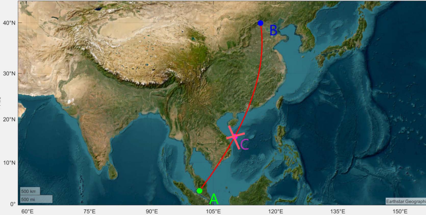
Figure 3: Flight path simulation
Assuming that an airplane flies from A to B and loses power and is lost at point C halfway through the flight, we divide its crash into two parts, before and after entering the water. Before entering the water, the force analysis diagram of the airplane is shown in figure 4
The formula for lift is:
where:
- ρis the density of the fluid, and for aircraft flight, it usually refers to the density of air.
- Sis the reference area, and for an aircraft, it is usually the planar area of the wing.
- CLis the lift coefficient, which depends on factors such as the shape of the object, the angle of attack, and the Reynolds number.
The resistance (D) in fluid mechanics can be calculated by the following formula:
where
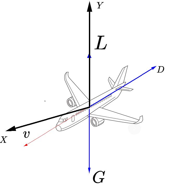
Figure 4: Force analysis of the airplane before entering the water
- CDis the drag coefficient, which depends on factors such as the shape of the object, the surface roughness, the Reynolds number of the fluid, and the flow state of the object relative to the fluid.
- ρis the density of the fluid, and its value is affected by environmental factors.
From this, the equations of Newton’s laws of motion in the horizontal and vertical direc- tions can be listed respectively:
Initial conditions:
Solved:
To facilitate further calculations, we shall not replace such analytical solutions with nu- merical ones. In this paper, we take the Boeing 777-200 model corresponding to MH as an example.After querying, we can see that the range of values ofCLis 0.5-0.6 and the range of values ofCDis 0.02-0.03, to facilitate the calculation, we take
H= 10, 000 m,CL= 0. 6 ,CD= 0. 02
, calculated by MATLAB : After entering the water, the force analysis diagram of the air- plane is shown in figure 5
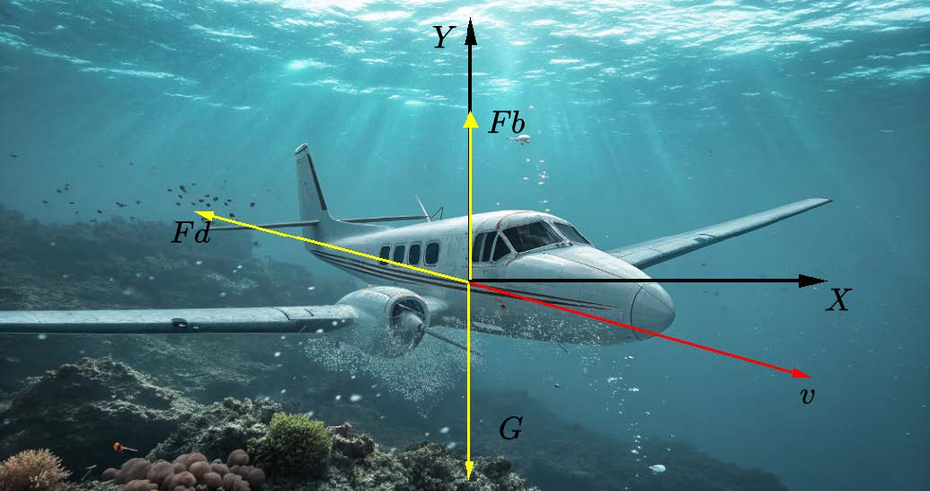
Figure 5: Force analysis of the airplane after entering the water
According to fluid dynamics, the drag force is calculated as follows:
where:
- Fdis the drag force acting on the object in water;
- ρis the density of water;
- Ais the projected area of the object in the direction perpendicular to the velocity.
- Cdis the drag coefficient, which depends on factors such as the object’s shape and surface roughness, and is generally determined through experiments;
The buoyancy forceFbexerted on an object immersed in a fluid can be calculated using the following formula based on Archimedes’ principle:
The time for the airplane to enter the water is neglected, and the equations of Newton’s
law of motion in the horizontal and vertical directions are listed, respectively: The value
of Cdthe range of 0.02-0.05, in order to facilitate the calculation, take
We calculate the optimal case (minimum drag coefficient in air and in water) and theworst case (maximum drag coefficient in air and in water) separately, the final possible crash area is calculated to be a sector-like area with a distance to the crash center between 14173.44-17256.77 m
| Table 2: Airborne fall modeling results | ||
|---|---|---|
| Optimal Situation | Worst Situation | |
| t | 77.5730 s | 74.0236 s |
| x | 17238.02 m | 14173 m |
7 Task 2: The representation of the probability density
Common sense suggests that the flight path of a crashed airplane in a real situation must not be purely linear, and the pilot must have adjusted the airplane’s flight attitude and an- gle. We believe that the maximum value of the airplane’s slope angle should be between 25-30° 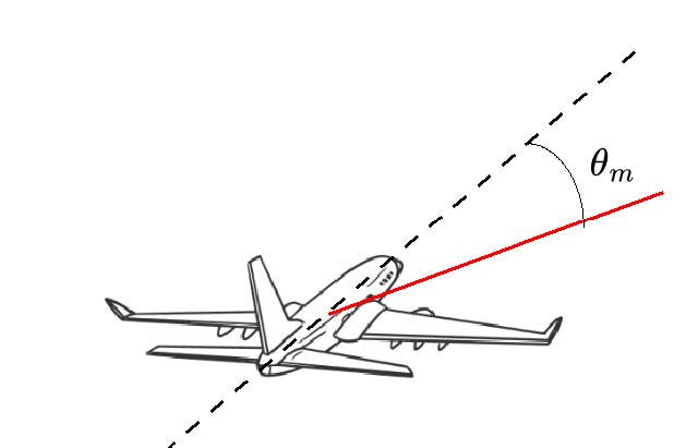
Figure 6: Schematic diagram of aircraft steering slope angle
This is because the angle of slope is an important parameter when an airplane isturning and directly affects the radius of the turn and the overload (G-force) The greater the angle of slope, the greater the overload to which the airplane and passengers are sub- jected. For example, a 30-degree slope angle produces an overload of about 1.15G and a 60-degree slope angle produces an overload of 2G. When the overload is too great and the pilot is unable to adjust in time, it can lead to tearing and disintegration of the airplane. At the same time, the prohibition of large angles is also to protect the normal traveling of the surrounding aircraft, so the Civil Aviation Administration stipulates that the maxi- mum slope angle is 25-30°. So we set up a model, here we take the accident place C as the origin, the direction of the initial speed of the flight as the y-axis, and the radial direction as the x-axis to establish a right-angled coordinate system, which is used to describe the flight trajectory of the aircraft in the limit of the maximum angle of gradient.
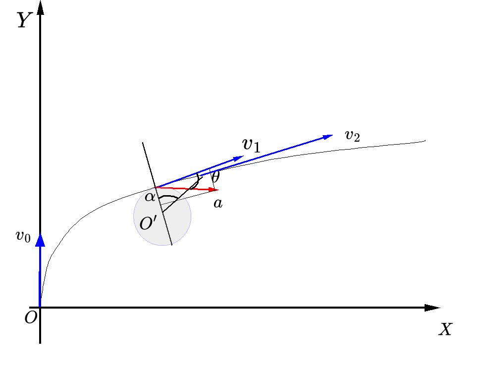
Figure 7: Schematic diagram of aircraft steering slope angle
Based on theanalysis of the forces in figure 7, it is clear that we can establish the system of equations
This equation is decomposed into velocity and radial direction by acceleration, and the knowledge of circular motion is used to get the amount of change in angular velocity and thus the trajectory of the airplane.ais taken to be 0. 15 g, andθis taken to be the maximum value of 30°, and so through MATLAB we get the relationship between the amount of side shift and our aforementioned maximum flight distance. Considering that the right turn and left turn are two completely symmetrical cases, and the maximum flight distance is customized so that we get the possible crash area of the aircraft. As shown in the figure 8
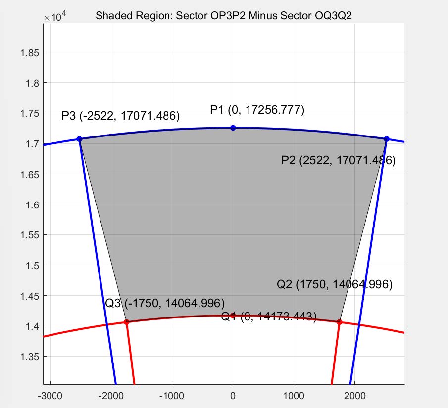
Figure 8: sector-like area map
Let’s review the airplane turn again, and we see that its physical scenario is exactly the same as the forces on the balls in the famous Galton board, and these same balls can only
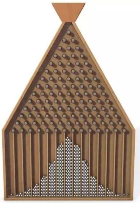
Figure 9: Galton version of the model
choose to turn left and right(figure 9). Therefore, we conclude that the probability of the airplane falling in this sector is not exactly the same, but conforms to the normal dis- tribution, with the y-axis in the forward direction of flight as the maximum point of the probability, and gradually decreasing to both sides of the x-axis. At the same time, consid- ering that the actual flight distance of the aircraft should also be between the maximum flight distance and the minimum flight distance, and in the statistical sense of conformity with the normal distribution, thus we established the XYZ three-dimensional coordinate system, with the Z-axis as the probability of the aircraft falling here, in order to facilitate the subsequent discussion.
From the binary normal distribution probability density function calculation equation
Significance of the five parameters of the two-dimensional normal distribution:
μx: the mean value ofx, indicating the center of the random variablex.
μy: the mean value ofy, indicating the center of the random variabley.
σx: the standard deviation ofx, the degree of dispersion ofx.
σy: the standard deviation ofy, the degree of dispersion ofy.
ρ: the correlation coefficient betweenxandy, denoting the correlation coefficient betweenxandy.xandy, indicating the degree of linear correlation between x and y.
Finally, we plotted the probability distribution as in Figure 10 11
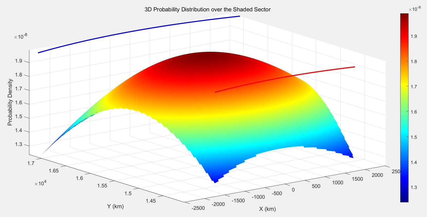
Figure 10: Probability Density Distribution I
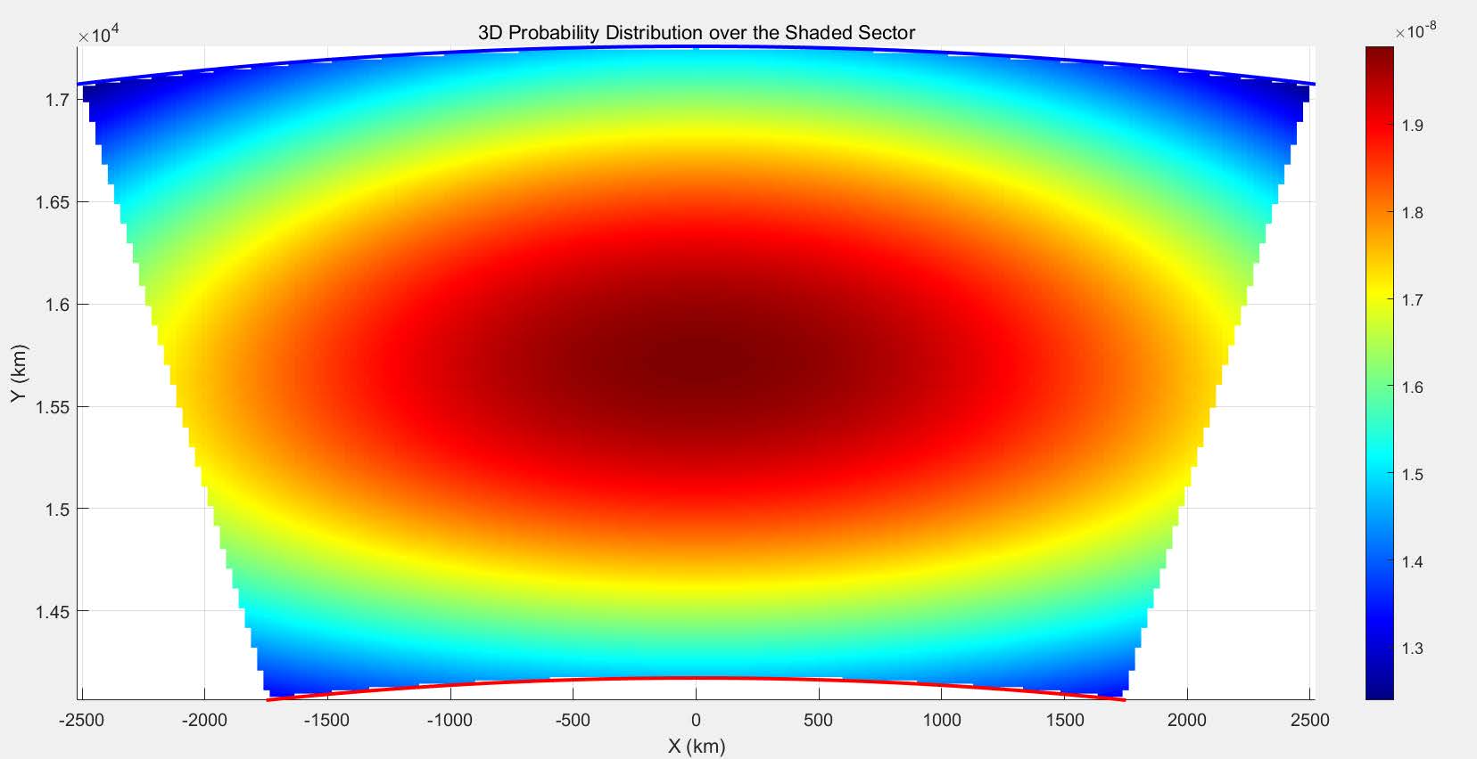
Figure 11: Probability Density Distribution II
8 Task 3: Optimization of Search and Rescue Strategies
According to the above part, we constructed a probability distribution based on the graph of the aircraft crash site, and below we will construct a reasonable model based on this probability distribution graph to determine the search and rescue pattern that is analyzed efficiently and has practical operability. For the construction of the search and rescue pattern, we are based on the characteristic attributes of the probability distribution map, we consider that the search intensity should be increased in the locations with higher probability to ensure the overall search effect is good, on this basis, we have to take into account the time of the search and rescue at the same time, to grasp the golden time of life of the search and rescue. According to this idea, we constructed the spiral search and rescue model and the Monte Carlo simulation-traveler search and rescue model.
8.1 Strategy 1: Spiral Search and Rescue Model
Modeling with the helix SAR model needs to consider the starting point of SAR, which we set as the highest point of probability and the helix center of the helix. In this model, we set up a polar coordinate system with the starting point of SAR as the origin:
a is the growth rate,r spiraldenotes the helix pitch, and a relationship exists betweenaand r spiral:
and according to the optical properties, we know that the general maximum radius of SAR of low-altitude SAR aircraft is 150m, and we set the maximum value of the pitch to be twice the maximum radius of the search and rescue, i.e., 300m, and the setting of the pitch increases according to the decreasing probability of the size of the crash (the range of the incremental increase is from 0 to 300m, and the range of the incremental increase is from 0 to 300m). The linear interpolation formula is used here:
where:
rspiral represents the radius of a point on the spiral.
rmin is the minimum radius of the spiral.
rmax is the maximum radius of the spiral.
θis the current angle (usually measured from a certain starting angle).
θmin is the angle corresponding to the minimum radiusrmin.
θmax is the angle corresponding to the maximum radiusrmax.
so that this setting can meet the need to reasonably increase the search and rescue accu- racy in places with high probability and ensure a higher overall efficiency. In this model, we determine the critical points as the four symmetric vertices of the search and rescue range, when the search and rescue range of the aircraft covers these four symmetric ver- tices (figure 12),
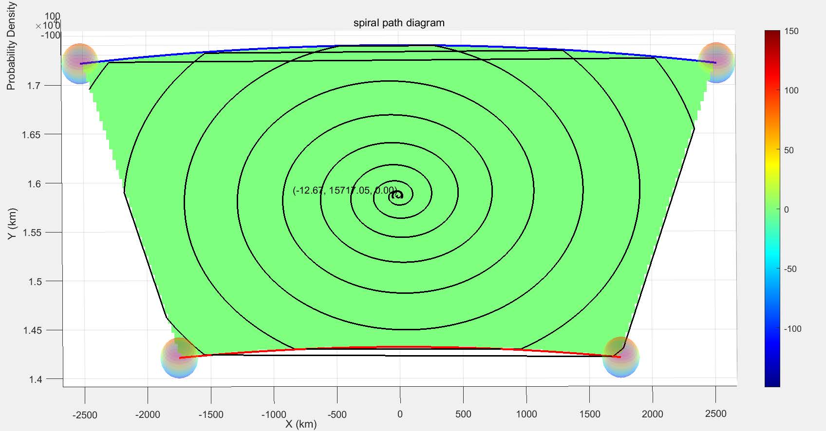
Figure 12: Spiral Search and Rescue Model
it means the end of the whole search and rescue process, which is also the end point of the spiral line, then we count the length of the spiral line , that is, the length of the search and rescue path:
8.2 Strategy 2: Monte Carlo simulation-traveler search and rescue model
In order to better adapt to the probability distribution of crashes in the search and rescue range, we first use Monte Carlo simulation to randomly generate a large number of possible crash points (100) based on the probability distribution, and then, after labeling on the graph, we use to build a traveler’s model, i.e., we use the simulated annealing algorithm to solve for the shortest path that connects a large number of crash points. In the process of Monte Carlo simulation, we randomly generated a set of 100 data points based on the principle of estimating probability by frequency under certain conditions,using the obtained normal distribution probability as a basis for path analysis. In the process of simulated annealing algorithm, we first randomly generate an initial solution, and then conduct a domain search around this initial solution to continuously generate new solutions,
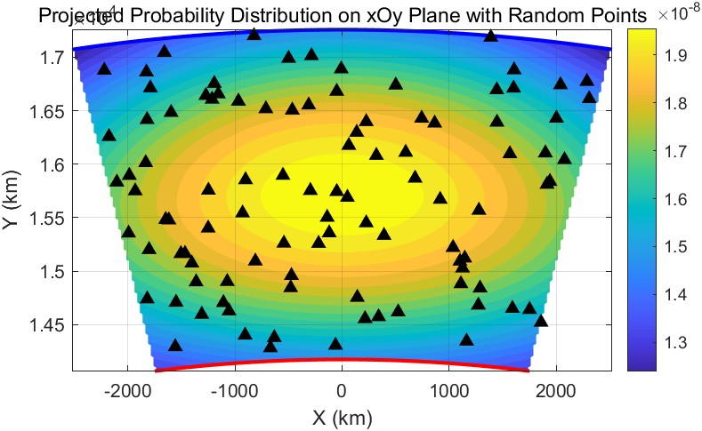
Figure 13: Monte Carlo Simulation Search and Rescue Model
where we set a certain acceptance criterion to eliminate inferior solutions with a certain probability as a way to avoid falling into a local optimum:
where:
- ∆Eis the difference between the objective function values of the new solution and the current solution.
- Tis the current temperature.
In the cooling process, we adopt an exponential cooling strategy to gradually reduce the temperature, narrow the search range,
where:
- Tkis the temperature at thek-th iteration.
- αis the cooling rate(0< α <1).
Here the initial temperature is set to 5000 degrees, the minimum temperature is set to 1 × 10 −^10 degrees, the cooling rate is set to 0.99, and the maximum number of iterations is set to 10,000, and finally converge to a better solution. Since the search and rescue pro-
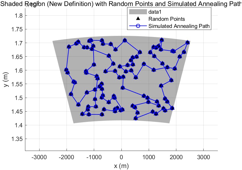
Figure 14: Simulated Annealing Algorithm Search and Rescue Model
cess cannot be based solely on the consideration of the shortest distance traveled and the highest probability of encounter with the downed aircraft, it must also be recognized that terrain and search and rescue capabilities have an impact on the success rate of search and rescue. We therefore define a functionλ, which we may refer to as the SAR intensity. This function is obviously proportional to the search radius of our search and rescue aircraft and the degree of information unimpeded, and the complexity of the undersea terrain, the harshness of the weather is inversely proportional. And the worse the environment, the lower the probability of successful search and rescue will be, so we introduce a function f(λi)from its extension, the expression can be as follows:
Clearly the probability of being saved is 1 whenλi= 0, and it is almost impossible to be saved whenλitends to infinity. This is consistent with our intuition. We therefore expect the following condition to be satisfied:
Pi is the probability that the rescue plane meets the crashed plane.P is the probability that the crashed plane is successfully rescued.S is always the shortest path.
9 Sensitivity analysis
9.1 Analysis of the effects of ocean currents
As the airplane crashes in the ocean, it will inevitably be affected by ocean currents, which generate shear forces that act on the seabed and push the wreckage of the airplane to move. Therefore, the crash area of the crashed aircraft no longer conforms to our afore- mentioned Gaussian distribution, and its probability center will inevitably shift towards the direction of the movement of the ocean currents. The effect of the ocean currents mov-
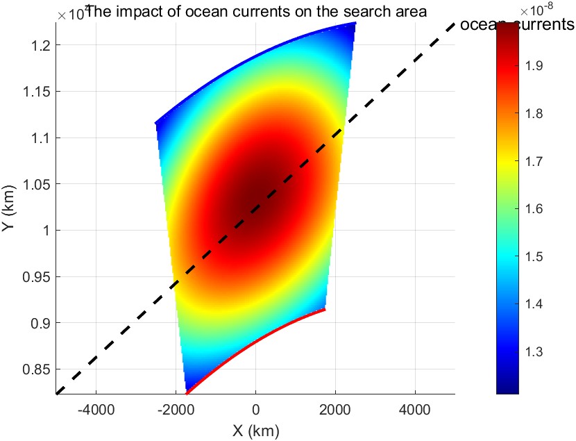
Figure 15: Actual probability plot with ocean currents
ing towards the northeast on our normal distribution is shown in the figure 15. The effect of the currents causes deformation and expansion of our search area, but the helix search method and the simulated annealing method based on Monte Carlo simulation are still valid because we can determine the final search and rescue route by predicting the effect of the currents on the probability distribution.
9.2 Analysis of the effects of changes in air density with altitude
Table 3: U.S. Standard Atmosphere Air Properties - SI Units (0 - 10000m)
| Height Above Sea Level ( h ) (m) | Density ( \rho ) (kg/m³) |
|---|---|
| 0 | 1.225 |
| 1000 | 1.112 |
| 2000 | 1.007 |
| 3000 | 0.9093 |
| 4000 | 0.8194 |
| 5000 | 0.7364 |
| 6000 | 0.6601 |
| 7000 | 0.5900 |
| 8000 | 0.5258 |
| 9000 | 0.4671 |
| 10000 | 0.4135 |
As shown in table 3, the air density is not constant, it increases as the altitude de- creases, which is extremely inconsistent with our previous take ofρ= 0. 8 kg/m^3. In order to determine the range of the crash site of the crashed airplane under the consideration of the change of air density, we carried out further calculations.
where:
- ρ 0 = 1. 225 kg/m^3 is the air density at sea level (under standard atmospheric condi- tions).
- L= 0. 0065 K/mis the vertical temperature gradient.
- T 0 = 288. 15 Kis the temperature at sea level.
- g 0 = 9. 80665 m/s^2 is the standard gravitational acceleration.
- M= 0. 0289644 kg/molis the average molar mass of air.
- R= 8. 31447 J/(mol·K)is the gas constant.
The law of air density variation with altitude is well studied, and ISA model can help us to solve this problem, we modifyρin the differential equation 5 toρ(y), where the functional expression is the famous ISA model, and then we unfold the calculation, and get the following results The final probability distribution does not change much from the previous one, this is because the deviation of the maximum distance is only (17658.4 − 17256.77)/17256.77 = 2.32%
Table 4: Analysis of the effects of changes in air density with altitude
| ( \ρ = 0.8 , {kg/m}^3 ) | ( \ρ ) varies with ( h ) |
|---|---|
| ( X_{\max} ) | ( 17238.02 , m ) ( 17658.4 , m ) |
| ( X_{\min} ) | ( 14173 , m ) ( 15974.8 , m ) |
, and the error of the shortest distance is 12.7%, which is represented in the graph as an increase in the scope of the search and the difficulty, but is still concentrated in the central area. At this point the two search and rescue models we proposed are still valid.
9.3 Analysis of the effects of lateral wind effects
In practice, we consider the influence of lateral wind, which can make the actual crash site deviate from the theoretical crash site by a certain distance. Taking the Boeing 777-200 as an example, we first calculate the force area of the airplane for lateral wind
and get the total analytical equation
Based on the analytical equation of the calculated force area, we bring in the wind load formula to calculate the wind force
where:
0.5ρv^2 is the dynamic pressure of the airflow (unit: Pa).
Ais the windward area of the object in the direction perpendicular to the wind direction (unit:m^2 ).
Cdis the wind load coefficient, which is related to the shape of the object, surface roughness and airflow characteristics.
The wind load factor for the lateral wind of an aircraft is known to be approximately 1- 1.3 (1.2 in this case). With the calculated analytical equation of wind force, we plotted the function line of the change of offset with the turn angle (roll angle) after 77. 573 s(figure 16)
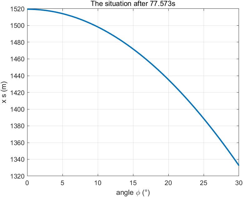
Figure 16: Plot of offset as a function of turning angle (angle of slope)
and based on the function line of the change of offset with the turn angle (angle of slope), we plotted the actual probability of crash distribution in figure17
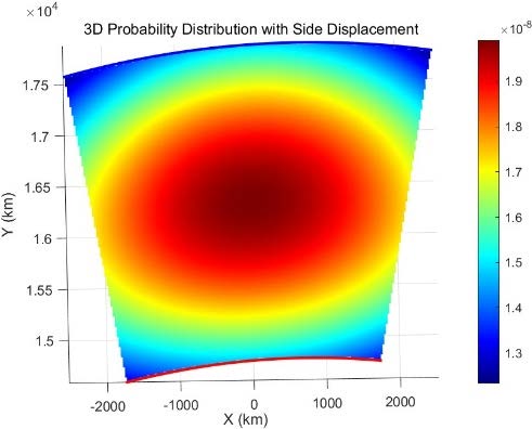
Figure 17: Actual probability plot with lateral wind influence
10 Conclusions
In addressing this problem, we simulated the disappearance of an aircraft over water by structuring the analysis into three primary modules: the physical model of the aircraft crash, the density probability distribution model, and the search and rescue model. To develop the physical model of the aircraft crash, we accounted for the complex forces exerted on the aircraft both during its flight over water and upon impact with the wa- ter’s surface. Utilizing the parameters derived from the physical model, we constructed a density probability distribution model that incorporates multi-dimensional probabil- ity distributions and factors in the actual crash range of the aircraft. Building on this density probability model and leveraging established search techniques, we devised two efficient search and rescue patterns, evaluating their respective applicability and oper- ational effectiveness. Additionally, we conducted extensive testing of the model under various scenarios, including mid-air disintegration of the aircraft, variations in air den- sity with altitude, and the influence of crosswinds. Our findings indicate that employing spiral search patterns and shortest-path planning based on probability-simulated points optimizes search efforts, ensuring comprehensive area coverage while enhancing overall search and rescue efficiency. These approaches also offer valuable insights and strategic direction for future search and rescue operations.
11 Strengths and weaknesses
11.1 Strengths
- The model is based on the probability of analysis, is relatively accurate, can effec- tively save search and rescue time and increase the effect of search and rescue, grasp the key time of rescue, and can bring more benefits for the rescue to save more lives of individuals.
- Considering the search and rescue schemes of different models, the scheme is more universal and more adapted to the actual situation.
- In the sensitivity analysis part, we consider many practical situations of rescue on the ocean, which are based on the unique geographic characteristics of the ocean, such as ocean currents, the unique air density of the ocean, etc. These considerations make our model more usable and adaptable to the actual situation.
11.2 Weeknesses
- It is difficult to fully consider the specifics of aircraft disintegration and dispersal, and the impact of the diversity that may result from the disintegration of an aircraft.
- The probability of rescue/probability of discovery/intensity of search and rescue by rescue aircraft is difficult to quantify.
12 References
[1].Anderson, J. D. (2010).Modern compressible flow: With historical perspective(3rd ed.). McGraw-Hill Education.
[2].Bertin, J. J., & Cummings, R. M. (2009).Aerodynamics for engineers(5th ed.). Pear- son.
[3].Box, G. E. P., Jenkins, G. M., & Reinsel, G. C. (2008).Time series analysis: Forecast- ing and control(4th ed.). Wiley.
[4].Clancy, L. J. (1975).Aerodynamics. Pitman Publishing. [5].Cook, M. V. (2013).Flight dynamics principles: A linear systems approach to air- craft stability and control(3rd ed.). Butterworth-Heinemann.
[6].Etkin, B., & Reid, L. D. (1996).Dynamics of flight: Stability and control(3rd ed.). Wiley.
[7].Feynman, R. P., Leighton, R. B., & Sands, M. (2011).The Feynman lectures on physics, Vol. II: Mainly electromagnetism and matter. Basic Books.
[8].Kirkpatrick, S., Gelatt, C. D., & Vecchi, M. P. (1983). Optimization by simulated annealing.Science, 220(4598), 671-680.https://doi.org/10.1126/science.220.4598.671
[9].Metropolis, N., Rosenbluth, A. W., Rosenbluth, M. N., Teller, A. H., & Teller, E. (1953). Equation of state calculations by fast computing machines.The Journal of Chemi- cal Physics, 21(6), 1087-1092.https://doi.org/10.1063/1.1699114
[10].Shevell, R. S. (1989).Fundamentals of flight(2nd ed.). Prentice Hall. [11].Tannehill, J. C., Anderson, D. A., & Pletcher, R. H. (1997).Computational fluid mechanics and heat transfer(2nd ed.). Taylor & Francis.
[12].Young, D. F., Munson, B. R., Okiishi, T. H., & Huebsch, W. W. (2010).A brief intro- duction to fluid mechanics(5th ed.). Wiley.
Appendices
SEARCH AND RESCUE PLAN
To: MCM office
From: MCM Team 12345678
Subject: MCM
Date: January 21, 2025
Today, I stand here with a heavy heart to discuss an important issue concerning avi- ation safety with all of you. In recent years, several incidents of commercial aircraft dis- appearances, particularly the MH370 tragedy, have not only deeply saddened us but also prompted us to reflect on how to enhance the efficiency of maritime search and rescue through scientific methods, thereby saving more lives in future emergencies.
Our research goal is to develop a universal mathematical model to predict the possi- ble crash area of an aircraft after a maritime accident and to optimize search and rescue strategies. Traditional search and rescue methods have many limitations, and our model, by integrating physical modeling, probability distribution, and dynamic optimization, can significantly improve the success rate of search and rescue operations while saving manpower, material resources, and time costs.
During the research process, we divided the entire project into three main tasks. First, we established a physical model of the aircraft crash, considering the trajectory of the aircraft after losing power in the air and the forces acting on it upon entering the water. Second, through a probability density distribution model, we predicted the possible crash area of the aircraft and generated detailed probability distribution maps. Finally, we pro- posed two optimized search and rescue strategies: the spiral search and rescue model and the Monte Carlo simulation-based traveler search and rescue model.
Our model has broad applicability and can adapt to different search and rescue sce- narios and environmental conditions. For example, we considered the impact of ocean currents, changes in air density, and crosswinds on the search area, and continuously optimized the model’s accuracy through sensitivity analysis. These improvements make our model more practical and effective in complex maritime environments.
Lastly, I want to emphasize that aviation safety is our shared responsibility. We hope that this research will contribute to the safe development of the global aviation industry. We also look forward to collaborating with our colleagues to advance maritime search and rescue technology, ensuring the safety of every passenger.
Thank you